ML Interview Q Series: Dice Game Strategy: Optimal Stopping Decisions Using Expected Value

Browse all the Probability Interview Questions here.
Imagine you have a fair six-sided die and you are allowed up to two rolls. After the first roll, you can either accept that value or try again. The amount of money you receive is the value on the final roll you keep. What is the maximum price you would pay to play this game?
Short Compact solution
An efficient way to decide is to keep the first roll if it is greater than the expected value of rolling again. The expected value of any single roll on a fair six-sided die is 3.5. Therefore, if the first roll is 1, 2, or 3, it is lower than 3.5, so you should roll again. If it is 4, 5, or 6, you should stop and keep it. You get 1, 2, or 3 on the first roll with probability 1/2, and in that scenario, the expected value for the second roll is 3.5. You get 4, 5, or 6 on the first roll with probability 1/2, and the average of 4, 5, and 6 is 5. Putting this together:

Hence, you should be willing to pay up to 4.25 dollars to play this game.
Comprehensive Explanation
This game is an example of a decision problem with an optimal stopping rule. You can roll the die once, observe the outcome, and then choose whether to keep that roll or forfeit it in favor of a second roll. If you opt for the second roll, you cannot revert to the first roll’s value. The core principle is to compare the first-roll result with the expected value of rolling again.
The expected value of any single fair six-sided die roll is the average of all possible outcomes (1 through 6). That is:

When deciding whether to keep a first roll or proceed to roll a second time, you compare the first roll outcome against 3.5. Any roll below 3.5 is worse than the anticipated 3.5 on the next roll, so you would generally want to roll again. Any result above 3.5 is better than the expected return from trying again, so you would keep that.
Concretely, 4, 5, and 6 are higher than 3.5, while 1, 2, and 3 are lower. Thus, you have a 1/2 probability of rolling 1, 2, or 3 on the first try. In those cases, you would reject your first roll and receive a second-roll expected value of 3.5. Meanwhile, if you roll 4, 5, or 6 initially (probability 1/2), you keep the roll, which on average is 5 (since the average of 4, 5, and 6 is 5). Combining these probabilities and values gives an overall expected payoff of:

Thus, the fair price of the game is 4.25 because that is the average amount you can win if you follow the best strategy.
To illustrate the decision strategy in code, you could simulate it as follows:
import random
import statistics

def play_game(num_simulations=10_000_000):
    payouts = []
    for _ in range(num_simulations):
        first_roll = random.randint(1, 6)
        # Compare with 3.5 to decide
        if first_roll < 4:  # i.e., 1, 2, or 3
            second_roll = random.randint(1, 6)
            payouts.append(second_roll)
        else:
            payouts.append(first_roll)
    return statistics.mean(payouts)

estimated_value = play_game()
print(estimated_value)
If you run this simulation a large number of times, you will observe a result that converges around 4.25, matching the analytic solution.
Follow-up Question 1
How would the optimal threshold strategy change if the die was biased or had different probabilities for each face?

Follow-up Question 2
What if you had the option to roll the die more than two times, say three times?
When you can roll more than twice, you use backward induction to determine the expected value of each roll. For three rolls, you start from the last roll and move backward:
On the third (final) roll, you have no choice but to accept whatever value you get. Its expected value is the average outcome (3.5 for a fair six-sided die).
On the second roll, you decide whether to keep that outcome or move to the third roll. That threshold is determined by comparing the second-roll outcome against the expected value of the third roll, which is 3.5 for a fair die.
On the first roll, you decide whether to keep that outcome or move on to the scenario where you effectively have a “two-roll” game left. You calculate the expected value of that “two-roll” scenario in exactly the same manner you computed the original two-roll game. That expected value is 4.25 for a fair die.
Thus, you keep the first-roll result if it is above the expected value of proceeding to the second+third roll scenario; otherwise you roll again. Then on the second roll, you keep or re-roll based on the threshold.
This logic extends to any number of rolls nn, but the arithmetic can become more involved. Typically, dynamic programming is used: you compute the expected value from the final roll up to the first, deciding threshold rules at each step.
Follow-up Question 3
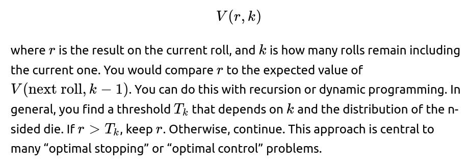
How can we generalize the approach to an n-sided die with k total rolls allowed?
The principle remains the same. You perform a backward calculation starting from the last roll. For each intermediate roll, you compare the current face value against the expected payoff if you were to forfeit the current value and proceed to the next roll. The difference is that you would compute the expected value for each roll by summing over all n faces. If k rolls are allowed in total, you effectively define a function:
Follow-up Question 4
How might risk aversion or utility theory change the optimal decision?
In real-world situations, people do not always maximize raw expected monetary value. Instead, they might maximize a utility function that is concave (for example, a logarithmic or square-root utility) to reflect risk aversion. If you are risk-averse, the subjective “value” of large payoffs grows more slowly than linear, and the threshold for deciding whether to roll again changes. You might settle more readily for a moderately high roll rather than gamble for a slightly higher return. The methodology is similar, but the comparison at each step is between:
“Utility of keeping current outcome” vs. “Expected utility if I roll again.”

Below are additional follow-up questions
If there were a fixed cost per roll, how would the optimal strategy change?

If there is a penalty for rolling a specific face (e.g., rolling a 1 results in a negative outcome), what happens?
Imagine a scenario where rolling a 1 actually yields a negative outcome, such as –2 dollars. This kind of penalty alters the expected value of a single roll. You would need to recompute the average outcome, taking the penalty into account:
If you roll a 1, you lose 2 dollars (instead of gaining 1).
For faces 2, 3, 4, 5, 6, assume normal payoffs.

What if the die is partially observable or has some hidden information aspect?
Consider a variant of the game where the first roll happens behind a screen and only partial information is revealed (for example, you learn whether the roll is odd or even but not the exact value). In such situations, you no longer know the exact outcome of the first roll, so you must compute an expected value based on the partial information available. For instance, if you only know that the hidden result is odd (1, 3, or 5), you would calculate the conditional expectation of that set (which is the average of 1, 3, 5 = 3.0) and compare it to rolling again (3.5 for a fair die). Conversely, if you know it is even (2, 4, 6), the conditional expectation is the average of 2, 4, 6 = 4.0, which might be higher than 3.5. The threshold decision is therefore based on partial knowledge rather than full knowledge of the roll, and you adjust your strategy accordingly.
A key pitfall is miscalculating these conditional expectations: if you don’t precisely compute the probabilities given your partial observation, you might adopt a suboptimal strategy. Another subtlety is if different partial observations have different prior probabilities or if some partial observations reveal more favorable sets of outcomes than others.
Does the correlation between the rolls (if any) affect the strategy?
If the outcomes of consecutive rolls are not independent (for instance, a mechanical die that is more likely to repeat the previous value, or a scenario where each face can only appear once), the entire analysis changes. For a standard fair die with independent rolls, computing the expected value is straightforward. But if the second roll depends on the result of the first roll, you must figure out the joint distribution of outcomes over two rolls.
For instance, suppose there’s a rule that after rolling a 6, the next roll is more likely to be a 1 (perhaps due to some mechanical bias). In this case, the expected value of the second roll is no longer a simple 3.5, and might be significantly lower. Therefore, if you get a 6 on your first roll, you might still keep it—even more strongly—because you know the next roll is likely to be quite poor. On the other hand, if your first roll is extremely low and you suspect the second roll might be high due to the correlation, you are even more incentivized to roll again. The difficulty is carefully computing the conditional probabilities for each possible outcome of the first roll so you can weigh the expected benefit of continuing.
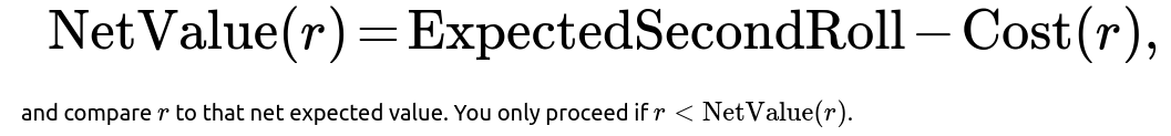
Could the game extend to a scenario where you must pay to access your second roll but that payment is determined by your first roll?
Another twist is a dynamic cost that depends on the first roll. For example, if the first roll is large, the second roll might cost you more to attempt. This could be a scenario in which the “house” charges a higher premium for the chance to improve on a good roll.
In such a situation, you can’t simply compare the first-roll value with a single fixed expected value for the second roll. You have to factor in how the cost scales with the first-roll result. If the cost becomes prohibitive for high rolls, it might still be worth paying for a second roll when you roll a 1, 2, or 3, but definitely not when you roll a 5 or 6, because the expected gain may be outweighed by the increased cost. A careful approach is to define a function:

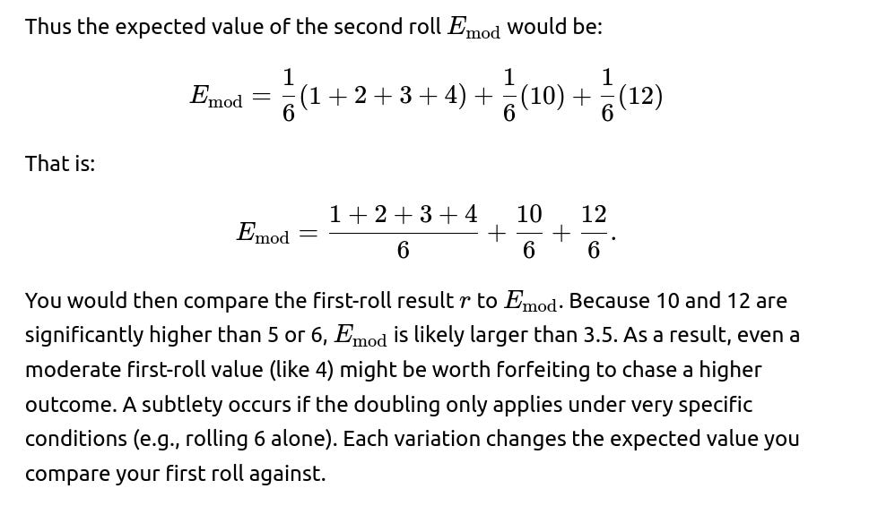
What if your payoff is doubled or multiplied if you roll above a certain threshold in the second roll?
In a modified version where, say, if the second roll is 5 or 6, the payoff is doubled, the straightforward computation of the second-roll expectation (3.5 for a fair die) no longer applies. Instead, you must calculate a new expectation. For the second roll:
Rolling 1, 2, 3, or 4 yields its face value.
Rolling 5 or 6 doubles the payout, so it becomes 10 or 12.

What if the game ends automatically if the first roll is below a certain threshold?
In some variations, you might not have a free choice to continue if you roll a 1. For instance, there could be a rule that says if you roll a 1 (or 1 or 2), the game ends immediately and you receive that outcome. This changes the expected value because you lose the opportunity to re-roll in those cases. When you do have a choice to roll again, you need to include in your computations the fact that some low outcomes automatically end the game.
A common pitfall is failing to incorporate how forced endings shift the distribution of possible final outcomes. Specifically, if rolling a 1 terminates the game, then in the analysis you would see that the probabilities for all other first-roll outcomes remain the same, but for the portion of the time you roll a 1, you forfeit the second roll entirely. Thus, the final expected value might be significantly lower than 4.25 because the advantage of re-rolling is lost in the worst cases.
What if you are allowed to see multiple dice outcomes at once and then choose which dice to keep?
A more complex spin involves rolling multiple dice in parallel and then choosing one to keep. Suppose you roll two dice simultaneously and can select one of them to keep or choose to re-roll both. The logic for an optimal strategy is more complicated: you look at the pair of outcomes you got, evaluate which die is better, and decide if that chosen value is above the expected value of another set of rolls. The threshold concept is still relevant, but you must compute the joint distribution over pairs of dice results.
For instance, if the pair is (6, 2), you will definitely choose the 6. Then you ask, “Is 6 better than the expected value of re-rolling both dice?” Because 6 is the maximum single-die result, you would normally keep it. But if there is some special bonus for rolling doubles in a future roll, you might weigh that possibility differently. If you roll (3, 3) and there is a premium on identical faces, you could use a new expected-value calculation that factors in that premium. The main pitfall is ignoring the correlation or synergy between the two dice outcomes. If you treat them as two separate single-die games, you might misjudge the benefits of re-rolling.
What about learning-based strategies using machine learning or approximate dynamic programming?
A more advanced angle is using simulated experiences or approximate dynamic programming to learn the best strategy. You could simulate many possible outcomes of multi-roll dice games, track the rewards, and update a policy function that decides when to stop or roll again. After enough simulations, the policy converges to an approximate (or exact) optimal threshold.
A subtle pitfall occurs if the state space is large (for instance, if you allow many rolls or have complicated rules). You might require more sophisticated function approximators (like neural networks) to represent the value function accurately. Hyperparameters—such as the discount factor or learning rate—could also affect performance. Overfitting can happen if you rely on a small number of simulations and incorrectly believe certain outcomes are more likely than they truly are.
When applying such learning approaches, you must be sure to:
Implement enough exploration so that all relevant states get sampled.
Set up your reward signals to properly reflect the payoff structure (and potential penalties).
Consider the computational cost of a large-scale simulation if the state space is extremely large (for example, 10-roll or 20-roll versions).
Failure to address these can lead to suboptimal learned policies.