
ML Interview Q Series: Discuss how Decision Trees contrast with Logistic Regression, emphasizing strengths, weaknesses, and typical usage scenarios.


📚 Browse the full ML Interview series here.
Comprehensive Explanation
Decision Trees and Logistic Regression are both commonly used models for classification tasks. Each has its distinct advantages, limitations, and underlying assumptions, making them suited for different kinds of problems. Below is a thorough exploration of these differences.
Conceptual Basis
Decision Trees operate by recursively splitting the feature space into subdivisions that aim to maximize the purity of each leaf node. The splitting criterion can be based on metrics such as Gini impurity or information gain. The final leaf nodes correspond to particular class predictions.
Logistic Regression is a parametric method that models the probability of a binary outcome as a logistic function of a linear combination of the input features. It fits a linear decision boundary but uses a non-linear transformation (sigmoid function) to bound probabilities.
Underlying Mathematical Formulation of Logistic Regression
A key formula for Logistic Regression is the sigmoid function that transforms any real value z into a range between 0 and 1:
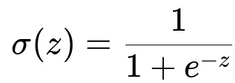
Here, z represents w^T x + b (in plain text: z = w transpose times x plus b). w is the weight vector, b is the bias term, and x is the feature vector. The function sigma(z) is often called the logistic or sigmoid function.
By applying this sigmoid function, Logistic Regression directly outputs the probability that a given example belongs to the positive (or "1") class.
Bias-Variance Profile
Decision Trees can have low bias but high variance, especially when grown to full depth. A deeper tree may overfit, capturing noise in the training data. Techniques such as pruning, ensembling, or regularization are typically applied to address high variance.
Logistic Regression has relatively low variance but can exhibit higher bias if the relationship between features and target is significantly non-linear. It is less prone to overfitting in its basic form when the number of features is not excessively large.
Handling Feature Interactions
Decision Trees naturally model feature interactions by splitting the feature space in a hierarchical way. As you go down the tree, each split can effectively represent an interaction of previously used splits with the next ones.
Logistic Regression in its basic linear form assumes that features contribute additively to the log-odds. It only models interactions if they are explicitly added as interaction terms or if non-linear transformations are applied.
Interpretability
Decision Trees can be interpreted by tracing the sequence of splits from the root node to a leaf node. The interpretability can diminish with very deep or complex trees, but a relatively short tree is often easy to understand.
Logistic Regression coefficients can be interpreted in terms of log-odds. A positive coefficient means increasing a particular feature’s value raises the probability of belonging to the positive class, while a negative coefficient implies the opposite. For many practitioners, this linear interpretation is straightforward to convey, especially in fields like healthcare or finance.
Dealing with Missing Values and Outliers
Decision Trees can handle missing values naturally by branching in ways that either skip missing data or treat them as a separate category. They are also relatively robust to outliers because splits are chosen based on purity criteria rather than raw values.
Logistic Regression typically requires missing data to be imputed, and outliers can disproportionately affect the parameters. Feature scaling or robust regression variants might be necessary when facing extreme values.
Computational Complexity
Decision Trees, in their most basic form, can be relatively fast to train for smaller datasets. But for large-scale problems, especially if many splits or features are considered, the training time can increase. Techniques like random forests or gradient boosted trees balance computation with predictive performance.
Logistic Regression is generally fast to train using gradient-based methods. In large-scale settings with high-dimensional data, logistic regression can be efficient, especially with optimized libraries or methods like stochastic gradient descent.
Practical Implementation in Python
Below is a simple example of how you might train both a Decision Tree and a Logistic Regression model using scikit-learn. This code illustrates the typical workflow, though in practice you would also include hyperparameter tuning, model evaluation, and so on.
from sklearn.datasets import make_classification
from sklearn.model_selection import train_test_split
from sklearn.tree import DecisionTreeClassifier
from sklearn.linear_model import LogisticRegression
from sklearn.metrics import accuracy_score

# Generate synthetic data
X, y = make_classification(n_samples=1000, n_features=10, random_state=42)

# Split into training and test sets
X_train, X_test, y_train, y_test = train_test_split(X, y, test_size=0.2, random_state=42)

# Train a Decision Tree
tree_model = DecisionTreeClassifier(max_depth=5, random_state=42)
tree_model.fit(X_train, y_train)
tree_predictions = tree_model.predict(X_test)

# Train a Logistic Regression
logistic_model = LogisticRegression(max_iter=1000, random_state=42)
logistic_model.fit(X_train, y_train)
logistic_predictions = logistic_model.predict(X_test)

# Evaluate accuracy
tree_accuracy = accuracy_score(y_test, tree_predictions)
logistic_accuracy = accuracy_score(y_test, logistic_predictions)

print("Decision Tree Accuracy:", tree_accuracy)
print("Logistic Regression Accuracy:", logistic_accuracy)
Potential Trade-Offs and Edge Cases
When deciding between these models, consider:
The complexity of the feature interactions. If the relationship is highly non-linear and complex, Decision Trees might capture interactions more efficiently, especially when used in ensemble methods.
The presence of high-dimensional data or scenarios where you need a well-calibrated probability. Logistic Regression might be favored for interpretability, speed, and straightforward probabilistic outputs.
The risk of overfitting. Decision Trees can overfit, so you might need techniques like pruning or ensembles. Logistic Regression can also overfit, but typically that happens with many correlated features or when the sample size is small.
Follow-up Questions
How do you decide when to prune a Decision Tree, and how might you prune it?
Pruning is usually done to control overfitting by stopping the tree from growing arbitrarily deep. You can use methods like cost-complexity pruning (also called minimal cost-complexity pruning in scikit-learn), which inspects subtrees and evaluates the trade-off between tree complexity (number of leaf nodes) and the training error. Another approach is setting hyperparameters like max_depth, min_samples_split, or min_samples_leaf to limit the tree’s depth or the minimum number of samples required at a node. Practically, you would combine these with cross-validation to find an appropriate complexity parameter.
Why might Logistic Regression fail to capture certain patterns in data?
Logistic Regression is fundamentally linear in the log-odds with respect to each individual feature unless you engineer non-linear features or interaction terms. If the underlying decision boundary is complex, the linear form can miss essential interactions or complex feature relationships. Feature engineering (like polynomial expansions or domain-specific transformations) is often required to help logistic regression capture these patterns. Additionally, if the features are highly correlated and you do not apply regularization or dimensionality reduction, the model can become unstable or overfit.
What if you need probabilities from a Decision Tree?
A single Decision Tree can produce probabilities by looking at the class proportions within each leaf. However, these probabilities might not be well-calibrated. Techniques such as Platt scaling or isotonic regression are sometimes used to calibrate the probabilities. Alternatively, ensemble methods like random forests often yield probabilities that tend to be more reliable, as they average predictions over many trees, effectively reducing variance.
When is it advantageous to use an ensemble of Decision Trees instead of a single tree or logistic regression?
An ensemble of trees (such as a random forest or gradient-boosted trees) can handle non-linear data distributions and complex feature interactions extremely well. These methods often outperform a single Decision Tree by reducing variance (in the case of random forests) or bias (in the case of gradient boosting). They can scale better with large data sets and often deliver better predictive performance than either a single tree or a plain logistic regression, although at the cost of interpretability and potentially longer training times.
What regularization techniques are used in Logistic Regression, and how do they help?
Common forms of regularization in Logistic Regression are L1 (lasso) and L2 (ridge).
L1 regularization adds a penalty proportional to the absolute value of the coefficients, encouraging sparsity in the coefficients (i.e., forcing some coefficients to become zero).
L2 regularization penalizes the sum of the squared coefficients, shrinking them toward zero but rarely making them exactly zero.
These penalties help control overfitting by reducing the magnitude of the coefficients in cases where the model might otherwise overfit to noise in the training data. Regularization can also improve numerical stability when dealing with highly correlated features.
How do missing values affect each method?
Decision Trees: Many implementations can handle missing values by either skipping those samples during the split, treating the missing values as a separate category, or using surrogate splits. This flexibility often makes decision trees more robust to missing data.
Logistic Regression: It typically requires a complete dataset. Missing values must be imputed or removed before training. If imputation is necessary, the quality of the imputation step can heavily influence the model’s performance.
Could you combine the interpretability advantages of Logistic Regression with a Tree-based method?
Yes, one approach is to build a small Decision Tree to capture non-linear interactions and then use the output of that tree (like the leaf index or path) as input features to a Logistic Regression. Another method involves using generalized additive models (GAMs), which are somewhere in between pure linear models and tree-based models. These frameworks allow you to approximate non-linearities in a more transparent fashion, preserving some interpretability while gaining modeling flexibility.