
ML Interview Q Series: Discuss various classification evaluation metrics and explain the contexts in which each one is most applicable.

📚 Browse the full ML Interview series here.
Comprehensive Explanation
Classification metrics assess how effectively a model distinguishes between classes. Different metrics highlight different aspects of performance, such as overall correctness, sensitivity to errors of certain types, or handling of imbalanced data. Below are the most commonly used metrics, along with explanations of when and why they are useful.
Accuracy
Accuracy is the ratio of correctly predicted outcomes (true positives + true negatives) to all predictions made. It is simple and intuitive, but it can be misleading when classes are highly imbalanced. In those cases, accuracy can remain high even if the model fails to identify minority class instances.
Precision
Precision is the fraction of predicted positive samples that are actually positive. It is particularly relevant in scenarios where false positives have a high cost. For instance, in spam detection, you want to avoid tagging legitimate emails as spam. Mathematically, it is often expressed as follows:
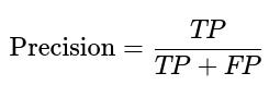
Here TP is the number of true positives, and FP is the number of false positives. This definition helps measure how "precise" or correct your positive predictions are, focusing on the cost of misclassifying negatives as positives.
Recall (Sensitivity)
Recall is the fraction of actual positive samples that are correctly predicted positive. It matters in situations where false negatives are more harmful, such as detecting a disease. The formula is:

Here TP is the number of true positives, and FN is the number of false negatives. A higher recall means fewer positive samples go undetected.
F1 Score
F1 combines precision and recall into a single metric by taking their harmonic mean. It helps when you need a balance between precision and recall or when you need a single figure of merit. It is usually used in imbalanced classification tasks to compare different models. The standard F1 score is:

Since it is the harmonic mean of precision and recall, F1 penalizes extreme imbalances between the two. If either precision or recall is very low, the F1 is also low.
ROC AUC (Area Under the Receiver Operating Characteristic Curve)
ROC AUC measures the probability that a randomly chosen positive example is ranked higher than a randomly chosen negative example. It captures the trade-off between the true positive rate and false positive rate across thresholds. It is usually a good measure of how well a model can distinguish between classes independently of class distribution or decision threshold, though it can be overly optimistic when dealing with severe class imbalances.
Precision-Recall AUC
Precision-Recall AUC is an alternate way to evaluate models especially in cases of heavily imbalanced data. It focuses on performance with respect to the minority class, and is often more informative than ROC AUC for tasks like anomaly detection or rare event prediction.
Confusion Matrix
A confusion matrix is not a scalar metric but an entire table that summarizes counts of true positives, false positives, true negatives, and false negatives. It gives a more detailed error analysis than a single summary metric. By looking at a confusion matrix, you can pinpoint exactly where the model is confusing certain classes.
Below is a minimal Python snippet demonstrating how to compute a confusion matrix for a binary classification problem:
import numpy as np
from sklearn.metrics import confusion_matrix

y_true = np.array([1, 0, 1, 1, 0, 1])
y_pred = np.array([1, 0, 1, 0, 0, 1])

cm = confusion_matrix(y_true, y_pred)
print(cm)  # array([[2, 0], [1, 3]])
When to Use Each Metric
Accuracy is fine when your dataset is balanced and all types of errors have a similar cost. Precision is crucial when the cost of false positives is high. Recall is crucial when the cost of missing positives is high (false negatives). F1 is good when the data is imbalanced, or when you want a single metric that balances precision and recall. ROC AUC is preferred when you want a threshold-independent measure and you have moderate or balanced class distributions. Precision-Recall AUC is most effective in heavily imbalanced scenarios, focusing on minority class performance.
How do you handle heavily imbalanced classes?
When the dataset has a high class imbalance, accuracy can become less meaningful because predicting the majority class alone can yield deceptively high accuracy. Strategies include:
Adjusting the decision threshold. Lower it to increase recall, though this may reduce precision (or vice versa). Using appropriate metrics like F1, Precision-Recall AUC, or Weighted F1 to better reflect performance for the minority class. Applying class-weighting or oversampling the minority class (e.g., SMOTE) to help the model learn from minority class instances more effectively. Using specialized sampling or ensemble methods such as Balanced Random Forests or undersampling the majority class.
Why might accuracy be misleading in some applications?
Accuracy can be misleading when one class vastly outnumbers the other. For example, if only 1% of the dataset is positive (rare cases), a model that predicts everything as negative achieves 99% accuracy yet has zero recall. In high-stakes applications like fraud detection or medical diagnosis, failing to catch rare positives can be detrimental.
When should you prefer Precision-Recall AUC over ROC AUC?
Precision-Recall AUC becomes more critical if you are focused on the performance of the minority (positive) class in highly imbalanced datasets. It gives a clearer picture of how effectively a model is identifying positives (precision and recall) rather than averaging across both classes. Conversely, ROC AUC considers the false positive rate on the negative class and can be overly optimistic when there is a large majority class.
What is the difference between macro-averaged and micro-averaged F1 scores?
Macro-averaged F1 computes F1 independently for each class and then takes their unweighted average, giving equal importance to each class. This is useful when each class is equally important regardless of frequency. Micro-averaged F1 aggregates contributions from all classes to compute the average metric; effectively, it weights each class proportionally to its size. This approach is helpful when you care more about overall performance than performance on minority classes.
How do you decide which metric is best for your problem?
Choosing a metric depends on the context, particularly the distribution of your target classes and the cost associated with different types of misclassifications. If data is balanced and all errors are equally important, accuracy can be a simple choice. If missed detections (false negatives) are costly, recall is paramount. If false alarms (false positives) are costly, precision is key. If you need a balanced view, F1 is a good summary. If you have imbalanced data and want to evaluate overall ranking performance, you may look at ROC AUC or Precision-Recall AUC depending on whether you prioritize majority class or minority class performance.
Below are additional follow-up questions
How would you evaluate performance in a multi-label classification scenario where each sample can belong to multiple classes simultaneously?
In multi-label classification, a single instance can have multiple positive labels at once. Common metrics like Accuracy or Precision/Recall for binary classification need to be adapted, as we do not just classify one label per sample but potentially several. Key approaches include:
Exact Match Ratio: Measures the proportion of samples for which all predicted labels match the true set of labels exactly. This is very strict and often yields low values because the model must get every label correct.
Hamming Loss: Evaluates how many labels are misclassified on average. It counts every pair of (instance, label) that is incorrectly predicted (missing a label that should be there or predicting a label that shouldn't).
Micro-Averaged F1: Aggregates true positives, false positives, and false negatives across all labels. This approach can work well when class frequencies vary significantly, as it weighs them by their frequency.
Macro-Averaged F1: Calculates the F1 score independently for each label and then averages them, giving equal weight to each label regardless of frequency.
A potential pitfall arises when some labels occur much more often than others. In that case, macro-averaging ensures rare labels get a fair share in the metric, whereas micro-averaging might overshadow rare labels with the contribution of frequent labels. In real-world multi-label use cases (e.g., tag prediction in content recommendation), it is crucial to decide which labels are more important and choose a suitable metric or combination of metrics accordingly.
What if your model's performance varies over time due to non-stationary data? Which metrics or strategies would you use to detect performance drift?
When data distribution evolves over time (known as concept drift), historical metrics may no longer accurately reflect current performance. Some strategies to detect and handle drift include:
Time Windows: Periodically calculate metrics such as Accuracy, Precision, Recall, F1, or AUC on the most recent data slices. Compare these with historical windows to see if performance deviates significantly.
Statistical Tests: Use hypothesis testing (e.g., Kolmogorov-Smirnov test) to compare feature distributions or label distributions between recent data and older data. A significant difference could indicate drift.
Drift-Specific Metrics: Some frameworks provide drift detection indicators (e.g., ADWIN) that signal if a model’s error rate is changing.
A potential edge case is when drift happens very gradually, making it harder to detect abrupt changes in metrics. Another subtlety arises if certain sub-populations of data begin to appear more frequently. While overall metrics might remain stable, performance on some sub-population could degrade significantly. Monitoring performance by segment or feature distribution is therefore essential for real-world applications where user behavior or data patterns shift over time.
How do you interpret a large multi-class confusion matrix (e.g., 10 or more classes) and diagnose poor performance using it?
A multi-class confusion matrix extends the binary confusion matrix structure to more rows and columns. Each row corresponds to the actual class, while each column corresponds to the predicted class. Interpreting it can be challenging with many classes, so specific steps include:
Normalize Rows: Viewing each row as percentages helps identify where the model confuses one specific actual class for another. If a particular row has high values in the wrong columns, it means the model consistently misclassifies that class.
Highlight Off-Diagonal Patterns: Systematic confusion might indicate that some classes have very similar features. For example, the model might confuse Class 2 and Class 7 often, suggesting an overlap in their data distributions.
Focus on Most Common Mistakes: Identify which pairs of actual and predicted classes show the highest misclassification counts. This might guide you to collect more data or engineer features that can better separate those classes.
Potential pitfalls include being overwhelmed by too many classes and focusing only on overall accuracy. Some classes might have extremely low recall, yet this is masked in the overall accuracy if that class is rare. Another subtlety is that certain "nearby" classes might be more acceptable confusions than unrelated classes (e.g., misclassifying a 'cat' as a 'lynx' might be less concerning than labeling it a 'car').
How would you design a cost-based metric when some misclassifications are costlier than others?
In many real-world applications, different errors incur different penalties. For instance, in credit scoring, approving a bad loan (false positive) might be more expensive than rejecting a good customer (false negative). You can incorporate these costs into a custom metric or objective function. A simplified cost function might look like:

Where c_fp is the cost of a false positive, and c_fn is the cost of a false negative, while fp and fn are the respective counts of those errors. In practice:
Estimating c_fp and c_fn: Requires domain knowledge. For credit scoring, you could estimate average financial losses for approving bad credit vs. lost revenue for rejecting good credit.
Hyperparameter Tuning: You can incorporate the cost function into your loss or set decision thresholds that minimize this cost rather than a standard metric such as Accuracy or F1.
Pitfalls: If cost estimates are unreliable or if they change over time, your cost-based metric might become obsolete quickly. It is also possible that focusing solely on cost can degrade user experience or fairness if certain user groups are disproportionately affected.
In practice, how do you balance conflicting requirements where business wants high Precision and regulators require high Recall?
This often arises in scenarios like compliance or fraud detection. The business side might not want too many false positives (for example, flagging legitimate transactions), while regulators might penalize missing suspicious cases (wanting fewer false negatives). Approaches to resolve this conflict include:
ROC or Precision-Recall Trade-Off: By examining your ROC curve or Precision-Recall curve, you can see how different threshold settings shift the balance between true positives and false positives. You can then choose a threshold that best meets both parties’ expectations.
Weighted F1 or Custom Metrics: In some cases, you might combine Precision and Recall with different weights to reflect the relative importance of each. If recall is more critical, you give it a higher weight.
Regulatory Sandbox Testing: In regulated environments, you might pilot new threshold settings or models on a subset of users or transactions and measure the real-world impact. This iterative approach can refine the balance between conflicting needs.
Potential edge cases occur if your data is extremely imbalanced, making it difficult to achieve both high precision and high recall simultaneously. Additionally, if either side pushes too far, it may impose operational burdens (e.g., too many manual reviews). The best real-world solution often comes from negotiation and careful threshold tuning, plus continuous monitoring to ensure that the chosen trade-off remains valid over time.
How would you handle threshold tuning in a scenario where you have multiple classes and each class has a distinct cost of misclassification?
In a multi-class setup, each misclassification type (predicting class i instead of class j) can carry a unique cost structure, rather than just “positive” or “negative.” Strategies for threshold tuning include:
One-vs-Rest Approach: Train a separate classifier for each class vs. all others. Each classifier then has its own decision threshold that you can adjust. You might penalize misclassifications into or out of each class differently. Finally, you combine their outputs to form the final multi-class label.
Cost-Sensitive Extension: If you have a direct cost matrix with dimension K x K for K classes, you can incorporate it into the training objective or post-processing step. After computing class probabilities, you can multiply them by the respective misclassification cost to choose the class that yields the lowest expected cost.
Practical Considerations:
Overfitting: If you tune thresholds too precisely on a small validation set, you may inadvertently overfit.
Changing Costs: Real-world environments might shift the cost structure, requiring frequent re-tuning or dynamic threshold assignment.
An edge case is when the model might be biased toward the most frequent or low-cost classes. If, for example, your cost matrix heavily penalizes mistakes in a minority class, the model might significantly alter how it classifies borderline cases for that class. This might drive up false positives in other classes, so you must be prepared to monitor global performance as well as class-specific cost metrics.
What strategies would you use when test data is expensive, and you only have limited labeled data to validate your classification metrics?
When labeled data is extremely scarce, evaluating classification metrics accurately becomes challenging:
Cross-Validation on Limited Data: Use techniques like stratified k-fold cross-validation to make the most out of your dataset. Stratification ensures each fold has a representative class distribution.
Active Learning: Iteratively choose the most uncertain or informative samples for labeling. By selectively labeling the most ambiguous points, you gain more insight into model weaknesses without needing to label the entire dataset.
Bootstrapping: Apply bootstrapping or repeated subsampling methods to estimate variability around metrics. While not a perfect replacement for a large dataset, it can yield confidence intervals that help gauge metric stability.
Synthetic or Semi-Supervised Methods: In certain cases, you might employ synthetic data generation for minority classes, or rely on semi-supervised learning to label large unlabeled sets. However, synthetic approaches risk introducing data that does not reflect real-world distributions if not carefully managed.
A subtle issue arises if your data collection process is itself biased (e.g., only certain samples get labeled). If you only sample “likely positives” for labeling in a heavily skewed scenario, your metrics might not reflect true performance. Another pitfall is over-reliance on synthetic expansions that deviate too far from the real-world domain.
How can you evaluate classification performance when you have partially observed ground truth labels?
Sometimes in real-world scenarios (e.g., user feedback systems), you only know if something is positive when users explicitly flag it, and silence might not necessarily be a true negative. This partial labeling complicates standard metrics:
Positive and Unlabeled (PU) Learning: This is a specific framework where you have definite positive examples but the rest are unlabeled rather than guaranteed negatives. There are specialized algorithms and estimation methods to adjust for unlabeled data potentially containing some positives.
Propensity Scoring: If you have a model of the label acquisition process, you can weight unlabeled instances according to how likely they would have been observed if they were truly positive or negative.
Careful Model Monitoring: Compare predicted positives against actual labeled positives over time, but be aware that some unlabeled items might be false negatives. One approach is to do occasional random checks of unlabeled data to see if it was truly negative or if it was a missed positive.
A hidden danger is underestimating or overestimating your false negatives because some unlabeled examples might be genuine positives that were not flagged. This can lead you to incorrectly conclude that your recall is higher than it actually is. Over time, you might implement a feedback loop to actively verify uncertain predictions, reducing the size of the unlabeled pool.