ML Interview Q Series: Efficient Large Model Training: Mini-Batch Gradient Descent Explained vs SGD & Batch

📚 Browse the full ML Interview series here.

SGD vs Batch Gradient Descent: Explain the differences between stochastic gradient descent (SGD) and full batch gradient descent. Why is mini-batch gradient descent generally preferred for training large models, and what are the trade-offs in terms of convergence speed and stability?

Below is a comprehensive and detailed explanation addressing the question about stochastic gradient descent (SGD) versus batch gradient descent, followed by potential follow-up questions (in H2 font) and their in-depth answers.

Understanding the Key Concepts

Stochastic gradient descent (SGD) and batch gradient descent are two distinct but related optimization strategies used to train machine learning models. The goal in both approaches is to find parameter values that minimize a chosen loss function. These methods differ in how they estimate the gradient of the loss function at each iteration.

Differences Between SGD and Full Batch Gradient Descent

Stochastic Gradient Descent (Classical Definition) Stochastic gradient descent, in its classical sense, processes one single data sample (or a very small subset, effectively size=1) at each iteration. For a dataset with many samples, a single update step involves computing the gradient of the loss function with respect to the model parameters on just this single sample, then updating the parameters accordingly. In more formal terms, if the dataset has samples indexed by i, the gradient of the loss function at iteration t on a single training example i can be represented as a gradient of the form

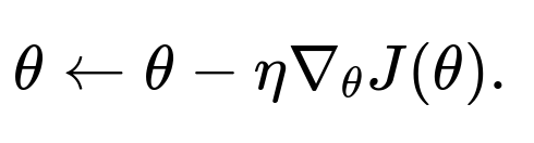
where (\theta) denotes the model parameters, and ( (x_i, y_i) ) is a single training example. After computing this gradient, an SGD update step for the parameters might look like

where ( \eta ) is the learning rate.

Full Batch Gradient Descent Full batch gradient descent computes the gradient using the entire dataset before performing a single update. This means, if the dataset has N examples, the gradient used in an update is an average (or sum) across all N samples. Formally,

Then the update step becomes

Here, the parameter update is made after considering all data points.

Why Mini-Batch Gradient Descent is Generally Preferred

Practical Efficiency Mini-batch gradient descent typically uses batches of a moderate size (for instance, 32, 64, 128, etc.). This approach balances computational efficiency and convergence speed. Processing a single sample at a time (classical SGD) can be highly variable, whereas computing the gradient across an entire massive dataset (full batch) is computationally expensive and can be slow to produce each update. Mini-batch gradient descent leverages the parallelization capabilities of modern hardware (e.g., GPUs), since gradients can be computed for multiple samples at once.

Smoother Convergence Using a mini-batch introduces less variance in the gradient estimate compared to purely stochastic (single sample) approaches. Although there is still some stochasticity due to the random sampling of a batch, the gradient estimate from a batch is more representative of the total dataset than the gradient from a single example. This leads to a smoother, more stable training curve than pure SGD, while still introducing enough randomness to escape sharp local minima.

Better Memory Utilization On hardware such as GPUs, vectorized operations over a small to moderate batch can be significantly faster than performing many single-sample operations. Also, storing very large batches might exceed memory limits, whereas a moderately sized batch is often the sweet spot.

Trade-Offs in Convergence Speed and Stability

Stochastic Gradient Descent (Classical) Pros and Cons Pros: Allows very frequent parameter updates, which can lead to rapid initial convergence. Can explore the loss surface more randomly, sometimes helping to avoid local minima or saddle points.

Cons: High variance in gradient estimates can cause erratic parameter updates. It may need careful tuning of the learning rate to avoid divergence.

Full Batch Gradient Descent Pros and Cons Pros: Uses the exact gradient over the entire dataset for each update, so updates are directionally accurate in the sense that each step is fully informed by all data. Can converge steadily when the loss landscape is well-behaved, without the noisy fluctuations of stochastic approaches.

Cons: Extremely expensive for large datasets, since each gradient calculation passes over all samples. May require a large memory footprint, and each training iteration can be very slow.

Mini-Batch Gradient Descent Pros and Cons Pros: Provides a good compromise by using partial batches. The gradient estimate for each batch is less noisy than in pure SGD, while still retaining enough stochasticity to avoid poor local minima in complex landscapes. Computationally more efficient on hardware accelerators than pure SGD or full-batch approaches. Typically leads to faster real-world training times and a stable convergence path.

Cons: Requires some tuning of batch size. Too small a batch can still be noisy. Too large a batch can behave similarly to full batch with slow updates, and might require large memory. Can have local minima or saddle behavior that is partially alleviated by the moderate stochasticity but not as much as the single-sample approach, depending on the problem.

Because of these combined benefits—computational efficiency, stable yet still stochastically driven gradient estimates, good memory utilization—mini-batch gradient descent is overwhelmingly the preferred method for training large-scale deep learning models in practice.

How Does Learning Rate Selection Differ Between Full-Batch GD and Mini-Batch Methods?

In a mini-batch setting, the presence of gradient noise often suggests using slightly higher learning rates early in training than one might use in a full-batch setting. The gradient noise can help the model escape plateaus and narrow local minima. However, if the learning rate is too high, the added noise can destabilize training. Learning rate schedules (e.g., decaying learning rates over time or employing strategies like learning rate warmup and then decay) can be beneficial. In contrast, with full batch gradient descent, because the gradient is the “true” gradient of the entire dataset, you might need a stable, generally smaller learning rate to ensure convergence without oscillation.

Does Pure Stochastic Gradient Descent or Mini-Batch Gradient Descent Help Avoid Local Minima More Effectively?

Random fluctuations in the gradient can sometimes help jump out of shallow local minima or saddle points. Pure SGD provides the greatest amount of fluctuation (since it looks at individual samples), but mini-batch also maintains enough noise to help avoid certain pathological regions in the loss landscape. Practically, mini-batch is the usual approach because pure SGD can become too noisy, resulting in less stable and slower convergence in real-world training.

What Role Does Batch Size Play in the Generalization of Deep Models?

There is empirical evidence that smaller batch sizes tend to yield better generalization in some settings. A common hypothesis is that the added stochasticity or noise in the gradient updates acts as a form of regularization. Larger batch sizes might lead to sharper minima, which can sometimes hurt generalization. In practice, the difference may be problem-dependent; many large-scale tasks are trained with fairly large batch sizes due to hardware efficiency demands, and they still generalize well, especially when combined with appropriate regularization or training schemes. Often, techniques like gradient accumulation or adaptive learning rate schedules are used to mitigate adverse effects of large batch training.

What Implementation Details and Pitfalls Arise When Using Mini-Batches in Frameworks Like PyTorch or TensorFlow?

When using mini-batches, you typically shuffle the dataset at each epoch or maintain a shuffled index list to avoid correlated sampling. Failure to shuffle or randomize properly may yield suboptimal convergence. You must also ensure that your batch size fits into GPU memory. If it does not, you might have to reduce the batch size or use gradient accumulation (where partial gradients are accumulated over multiple sub-batches before making an update). Additionally, certain layers (like BatchNorm) have different behaviors or hyperparameters that can depend on batch size. For instance, extremely small batch sizes can lead to unstable estimates in BatchNorm if the mini-batch statistics are not representative.

A very simplified PyTorch snippet (purely illustrative) for mini-batch gradient descent might look like this:

import torch
import torch.nn as nn
import torch.optim as optim

model = nn.Sequential(nn.Linear(784, 128),
                      nn.ReLU(),
                      nn.Linear(128, 10))  # example MLP for e.g. MNIST

criterion = nn.CrossEntropyLoss()
optimizer = optim.SGD(model.parameters(), lr=0.01)

for epoch in range(num_epochs):
    for batch_x, batch_y in train_loader:  # train_loader returns mini-batches
        optimizer.zero_grad()
        outputs = model(batch_x)
        loss = criterion(outputs, batch_y)
        loss.backward()
        optimizer.step()

In this code:

• train_loader yields mini-batches of data (batch_x, batch_y).

• We zero out existing gradients, compute the forward pass, compute the loss, backpropagate (i.e., calculate gradients), and update the parameters with the optimizer step.

What Are Some Strategies to Stabilize or Speed Up Convergence in Mini-Batch Gradient Descent?

Momentum or Nesterov Accelerated Gradient Adding momentum helps smooth out stochastic gradients by accumulating a velocity term across iterations. This often provides faster convergence on convex and nonconvex problems alike.

Adaptive Learning Rate Methods Optimizers like Adam, Adagrad, RMSProp automatically adjust the learning rate for each parameter dimension based on the history of gradients. This can greatly help in training deep neural networks with sparse or complex parameter spaces.

Learning Rate Schedules Reducing the learning rate over epochs or steps can help the model stabilize once it’s closer to a local or global optimum. Schedules like step decay, exponential decay, or more sophisticated approaches (e.g., SGDR or one-cycle policy) can improve final convergence.

Regularization Techniques To ensure good generalization and stable convergence, you typically also consider weight decay (i.e., (L_2) regularization), dropout, or other methods that help prevent overfitting when using mini-batches.

All of these strategies are complementary to the batch selection approach, further justifying why mini-batch gradient descent is widely considered the default in deep learning practice.

Could Full Batch Gradient Descent Ever Be Preferable?

Full batch methods can sometimes be beneficial in simpler, smaller problems where the dataset is small enough that computing the entire gradient is not computationally intensive. In such cases, the full batch gradient might provide stable progress in each iteration without the overhead of random sampling or multiple updates. In many real-world large-scale settings, however, the cost of each update on the full dataset becomes a bottleneck.

Summary of the Differences and Preferences

Stochastic Gradient Descent (SGD) (1 sample at a time)

• Very noisy updates, potential for quick initial progress, tough to stabilize at scale.

Full Batch Gradient Descent (all samples at once)

• Very stable updates, potentially very slow iteration time with large datasets, memory-heavy.

Mini-Batch Gradient Descent (subset of samples per batch)

• Blends the best of both worlds: moderate noise, efficient implementation, good memory utilization, stable convergence.

In modern deep learning, the phrase “SGD” is often used interchangeably with mini-batch gradient descent. Despite this, conceptually, there is a distinction. However, in practical usage, people refer to “SGD” when they actually mean “mini-batch gradient descent.”

As such, mini-batch gradient descent is generally preferred for large-scale model training because it balances stability, computational efficiency, and memory usage, while still incorporating helpful stochasticity to navigate the loss landscape effectively.

---

Below are additional follow-up questions

What Are the Main Differences in Computational Graph Construction Between Batch GD and Mini-Batch GD, and Why Does It Matter?

When training using batch gradient descent, the entire dataset is typically processed in one large forward pass to compute the loss, then one backward pass over the entire dataset’s contribution to the loss. This means the computational graph encompasses all samples at once. In contrast, mini-batch gradient descent repeatedly constructs a smaller computational graph for each subset of data.

In modern frameworks like PyTorch or TensorFlow (using eager modes), the graph is dynamically built for each batch. Each pass over a mini-batch is more manageable in memory compared to processing the entire dataset at once. The difference matters because:

Memory Utilization When the dataset is large, building the full-batch graph can exceed memory limits, especially with big neural networks. In mini-batch mode, the memory footprint is proportionally smaller.

Implementation Flexibility Mini-batch training enables frequent parameter updates, which can be beneficial for faster iteration and debugging. The graph is also simpler to handle within data loaders and GPU parallelization.

Potential Pitfalls and Edge Cases If batch gradient descent is used on a very large dataset, you might run out of memory even if you conceptually can handle the full pass. Also, for extremely small mini-batches, overhead from constructing these graphs might become a bottleneck and reduce training throughput.

How Can Data Shuffling or Sampling Strategy Affect Convergence in Practice?

Shuffling your dataset every epoch or using carefully stratified sampling ensures that each mini-batch is drawn from a well-mixed set of samples. This can impact convergence as follows:

Bias in Gradient Estimates If the data loader is not shuffling properly, certain classes or patterns can appear together too frequently in specific mini-batches. This may cause biased gradient estimates that slow or disrupt convergence.

Data Order Effects Especially for non-convex problems, the initial batches can push parameters in certain directions that might or might not benefit final convergence. A good shuffle helps reduce systematic ordering biases.

Pitfalls and Edge Cases A common edge case is forgetting to shuffle, resulting in training that sees all examples of a single class in the first portion of an epoch. This can cause unstable learning dynamics. Another scenario arises in time-series or streaming data where naive shuffling can break the temporal relationships that might be essential for learning.

How Do Large Batches Influence the Numerical Precision of Gradients, and Why Is This Relevant for Deep Networks?

Modern deep networks often involve very large parameter counts, and floating-point precision can become a limiting factor:

Reduced Gradient Variance With large batches, the gradient estimate has lower variance, which in principle is helpful. However, smaller floating-point increments (especially in single-precision or half-precision) can make changes to weights less pronounced if the effective step size drops below machine epsilon.

Accumulation of Floating-Point Errors When summing over a large number of samples, floating-point errors can accumulate in the partial sums. This might lead to subtle instabilities or require a careful ordering of summation (e.g., Kahan summation) for better numerical accuracy.

Pitfalls and Edge Cases In half-precision training (float16), large batch sizes can degrade gradient fidelity, particularly if the sums involved exceed representable ranges or if small gradient updates underflow to zero. Techniques like loss scaling or mixed-precision training are used to mitigate this.

How Do We Approach the Choice of Optimizer Differently if We Use Pure SGD Versus Mini-Batch SGD?

Pure SGD using a single sample per update typically benefits from momentum-based methods or adaptive optimizers to smooth out high variance in the gradient. Mini-batch SGD can also benefit from momentum or adaptive methods, but the considerations differ:

Momentum vs. Non-Momentum With single-sample updates, momentum can drastically reduce noisy oscillations. In mini-batches, the variance is already partially reduced, but momentum often still accelerates convergence.

Adaptive Optimizers (Adam, RMSProp) Pure SGD may be more sensitive to the scale of features since each update is extremely noisy. Adam or RMSProp normalizes some of that noise by adapting the learning rate per parameter. For mini-batches, adaptive optimizers might help with sparse gradients or networks with different magnitude scales in different layers.

Pitfalls and Edge Cases Switching from one optimizer to another mid-training can cause sudden changes in training dynamics, especially if the learning rates are not carefully adjusted. Additionally, some advanced optimizers might require more memory overhead, which is another factor to consider for large mini-batches.

How Does the Notion of an “Epoch” Differ Across Stochastic, Mini-Batch, and Full-Batch Settings, and Why Might This Affect How We Evaluate or Save Models?

An epoch traditionally means one complete pass over all training samples. However, the frequency of parameter updates during one epoch varies with the gradient descent approach:

Full-Batch One epoch corresponds to exactly one update step, since the entire dataset is processed as a single batch. Model checkpointing or validation after each epoch provides minimal insight into early-phase learning because there are very few parameter updates within an epoch.

Mini-Batch One epoch may consist of many mini-batch updates. You can evaluate or save the model more frequently—e.g., after every few mini-batches. This gives finer control and potentially quicker feedback on training progress.

Pure Stochastic (Batch Size = 1) Potentially the largest number of updates in one epoch. Each sample leads to a gradient update. Validation or checkpointing can occur much more frequently. However, doing so too often can be time-consuming.

Pitfalls and Edge Cases When switching from a smaller batch size to a larger one, you might mistakenly keep the same number of epochs in your training plan. The total number of parameter updates becomes drastically different, so “epoch-based” comparisons can become misleading. Some practitioners instead focus on total steps or total gradient evaluations, which may be a more uniform measure across different training strategies.

What Are the Potential Advantages and Drawbacks of Using Extremely Small Mini-Batches for Very Large Datasets?

Advantages Extremely small mini-batches (like 2, 4, or 8 samples) introduce significant stochastic noise, which can help escape saddle points or certain minima. This might improve generalization if the problem benefits from noisy gradient signals. Also, smaller batches can reduce memory usage, enabling deeper or wider models within the same hardware constraints.

Drawbacks High variance in gradient estimates often leads to slower convergence. A small mini-batch can also reduce GPU utilization efficiency because modern GPUs thrive on larger matrix operations. Moreover, layers like Batch Normalization might produce inaccurate statistics if the batch is too small.

Pitfalls and Edge Cases If your dataset has large intraclass variance, each tiny batch might not represent all classes or data diversity well. You also run the risk of partial overfitting to the few samples in each batch. Another subtle pitfall is that small-batch training can lead to extremely spiky learning curves, which makes hyperparameter tuning (e.g., learning rate, momentum) more challenging.

Could We Interleave Different Gradient Computation Strategies Within One Training Cycle, and Would That Offer Any Benefit?

Some advanced research ideas propose mixing strategies, for instance performing a few iterations of small-batch (or single-sample) SGD to explore the loss surface, then switching to a larger batch for more stable updates. The theoretical rationale might be:

Exploration Phase Small or single-sample updates to escape local minima or saddle regions.

Exploitation/Stabilization Phase Larger batch updates once the model is near a promising region, leveraging more accurate gradients.

Pitfalls and Edge Cases There’s a risk of overhead from constantly switching batch sizes or from re-initializing certain layer statistics (BatchNorm). The complexity of implementing a dynamic batch strategy can also be high. Empirically, while certain specialized tasks may benefit, standard mini-batch training with a well-tuned learning rate schedule often performs comparably without the added complexity.

What Are Some Practical Strategies for Performing Distributed Mini-Batch Gradient Descent in Multi-GPU or Multi-Node Environments?

Gradient All-Reduce In frameworks like PyTorch’s DistributedDataParallel, each GPU processes a distinct subset of the mini-batch, computes partial gradients, and then averages them across all processes before completing the update step. This is typically referred to as “data parallelism.”

Synchronous vs. Asynchronous Updates Synchronous training ensures all workers finish computing their gradients before an update step. Asynchronous methods allow updates without waiting for slow nodes, which can speed up iteration but introduces gradient staleness issues.

Pitfalls and Edge Cases Communication overhead can become the bottleneck if the compute to communication ratio is poor. Also, differences in hardware or network speeds across nodes can lead to load imbalance. Large, distributed batch sizes might degrade generalization if not managed with appropriate learning rate scaling strategies.

How Do Batch-Normalization Layers Behave Differently in Full-Batch vs. Mini-Batch Training?

In standard training with mini-batches, Batch Normalization computes mean and variance for each mini-batch. In full-batch training, a single batch is the entire dataset, so the normalization statistics become the global dataset mean and variance in every iteration. This leads to the following points:

Variance and Mean Estimates With full-batch updates, BN’s running estimates effectively match the global dataset statistics, so there’s little difference between training-time and inference-time stats. In mini-batch mode, the running estimates gradually converge to approximate dataset-level stats.

Pitfalls and Edge Cases Full-batch updates with BN can be stable, but if the dataset is extremely large, it can create memory issues. Also, if you shift from mini-batch to full-batch training mid-run, your BN layers might need re-initialization of their running mean and variance. In small-batch scenarios, BN can become unstable if each batch is not representative enough.

How Do We Handle Datasets That Are Too Large to Fit Into Memory at Once When We Want to Do Mini-Batch Gradient Descent?

Streaming or Iterative Loading You can stream data from disk or a distributed filesystem in mini-batches without ever loading the entire dataset into memory. Tools like PyTorch’s Dataset + DataLoader handle this with custom iterators.

Sharding and Preprocessing In distributed setups, you might shard the dataset across multiple nodes. Each node only loads its partition of the data, and partial gradients are combined. Proper randomization across shards is important to avoid bias.

Pitfalls and Edge Cases Data pipelines can become a bottleneck if not carefully parallelized or cached. Also, if sharding is not done randomly, certain nodes might only see a subset of classes or patterns, thus harming overall convergence. Monitoring data throughput is crucial: if your GPU utilization is low, you may need to optimize the data-loading pipeline.