ML Interview Q Series: Ensuring Backpropagation Correctness via Numerical Gradient Checking

📚 Browse the full ML Interview series here.

28. Why is gradient checking important?

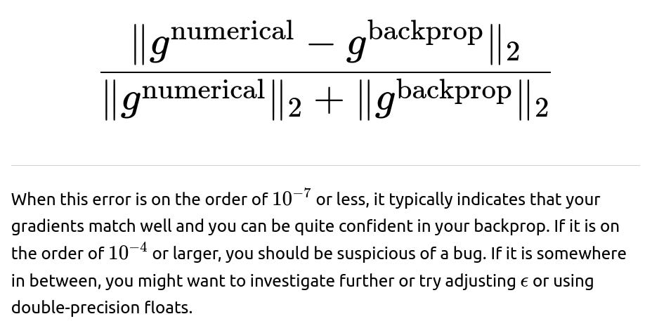
Gradient checking is a crucial technique used to verify the correctness of the backpropagation implementation in machine learning models, especially neural networks. In a typical training process, backpropagation computes analytical gradients of the loss function with respect to model parameters. If there is any error in the gradient computation—for example, a mistake in indexing, an off-by-one error, or an incorrect partial derivative—training can fail to converge or can lead to subtle bugs that are hard to detect. Gradient checking provides a way to numerically approximate the gradients and compare them with the analytically computed gradients from backpropagation. If the two match closely (within a small tolerance), it increases the confidence that your backpropagation is implemented correctly. If they diverge significantly, it signals an implementation error or numerical instability issues.

Gradient checking works by computing finite difference estimates of the gradient. Specifically, for each parameter dimension, you perturb that parameter slightly in the positive and negative directions and measure the changes in the cost (or loss) function. This numerical estimate is then compared to the analytically derived gradient. Because gradient checking is computationally expensive, it is usually applied on smaller test problems or on a random subset of parameters rather than the entire set in large models.

Below is an extensive discussion of the underlying concepts, how to do it in practice, potential pitfalls, and typical follow-up questions you might encounter in a rigorous machine learning interview.

Understanding the Concept of Gradient Checking

Reasons Why Gradient Checking is Important

It helps in detecting subtle implementation mistakes. Even if the loss decreases, it might be decreasing for the wrong reasons, or you might be using a learning rate that accidentally hides small mistakes in the gradient. Gradient checking helps isolate these errors.

It instills confidence in your training routine. Models such as deep neural networks rely heavily on correct gradient calculations. An error in the gradient might completely undermine training, especially for architectures with multiple submodules or custom operations.

It can reveal numerical stability problems. If your function is ill-conditioned or your network outputs become extremely large or small, gradient checking might show large discrepancies. This could be an early hint to incorporate better initialization, more stable activation functions, or proper normalization techniques.

It is a good practice for debugging. Although not used in production due to its computational expense, gradient checking is widely used in debugging phases, especially when building custom layers, advanced architectures, or specialized cost functions.

Steps to Implement Gradient Checking in Python

One typical approach to gradient checking in Python (using a pseudo deep learning model) might look like this:

import numpy as np

def compute_cost_and_gradients(theta, X, y):
    """
    This function computes:
    1) The cost J(theta)
    2) The gradients w.r.t. the parameters in theta via backprop
    """
    # Hypothetical cost and gradients computation
    # Replace with actual forward and backward passes.
    cost = np.sum(theta**2)  # Simplified cost
    grad = 2 * theta         # Simplified gradient
    return cost, grad

def gradient_checking(theta, X, y, epsilon=1e-4):
    # Compute the cost and gradient from backprop
    cost, grad_analytic = compute_cost_and_gradients(theta, X, y)

    grad_numerical = np.zeros_like(theta)

    for i in range(len(theta)):
        theta_plus = np.copy(theta)
        theta_minus = np.copy(theta)
        theta_plus[i] += epsilon
        theta_minus[i] -= epsilon

        cost_plus, _ = compute_cost_and_gradients(theta_plus, X, y)
        cost_minus, _ = compute_cost_and_gradients(theta_minus, X, y)

        grad_numerical[i] = (cost_plus - cost_minus) / (2 * epsilon)

    # Compute the difference
    numerator = np.linalg.norm(grad_numerical - grad_analytic)
    denominator = np.linalg.norm(grad_numerical) + np.linalg.norm(grad_analytic)
    difference = numerator / denominator

    return difference, grad_analytic, grad_numerical

# Example usage
theta_test = np.array([1.0, -2.0, 3.0])
X_test = None   # Replace with actual data
y_test = None   # Replace with actual labels
difference, grad_analytic, grad_numerical = gradient_checking(theta_test, X_test, y_test)

print("Difference:", difference)
print("Analytical Grad:", grad_analytic)
print("Numerical Grad:", grad_numerical)

Common Pitfalls in Gradient Checking

Forgetting to reset random seeds. If your model or cost function is stochastic in any way (e.g., dropout, random weight initialization, data sampling), you should ensure consistent behavior in the cost function calls for θ+ϵ and θ−ϵ. Otherwise, the numerical differences might reflect randomness rather than a stable gradient.

Applying gradient checking on the entire dataset for large networks can be prohibitively expensive. It is typically enough to do it on a small subset of the data or a small set of parameters.

Having issues with regularization terms or additional losses that might not be accounted for in your cost function for gradient checking. Make sure the exact same cost function is used in both the forward pass for the numerical gradient and the backward pass for the analytical gradient.

What Happens If Gradient Checking Fails?

If gradient checking yields a large discrepancy, it indicates a probable bug in the implementation or numerical instability in the function. You should systematically investigate:

Whether the cost function used in the forward pass matches exactly what is used for the backward pass.

Whether every dimension in your gradient is being computed in the correct order. Common issues include shape mismatches, transposed dimensions, or mixing up row vectors and column vectors.

Whether there are missing terms in your gradient, such as partial derivatives for regularization components or custom activation terms.

Whether there is an order-of-operations mistake: sometimes you forget to multiply or chain a partial derivative with an upstream gradient in the chain rule.

Whether numerical overflow/underflow is happening for certain parameter values. Checking intermediate values in the forward pass can be illuminating.

Use Cases in Real-World Projects

In real-world software development, especially at scale, gradient checking is often not run for every training iteration. Instead, you might rely on it for:

Verifying newly implemented model architectures or custom layers. If you build a new layer from scratch or define a new cost function, run gradient checking to ensure correctness before hooking it up to large-scale training.

Verifying learning frameworks. Libraries such as PyTorch and TensorFlow handle the majority of backpropagation automatically. But whenever you write custom autograd functions or lower-level GPU kernels, gradient checking can validate your approach.

Faster debugging cycles. When your loss is not decreasing in a proof-of-concept model or you suspect some strange behavior in training, gradient checking can quickly confirm or rule out gradient correctness as the source of the problem.

Below are some additional follow-up questions and detailed answers you might encounter.

How exactly is the numerical gradient computed and why does it work?

The numerical gradient is based on finite differences. The key idea relies on the definition of the derivative for a single-variable function in calculus. For a function f(x), the derivative at point x is the limit:

When do you do gradient checking in practice?

Gradient checking is most valuable in the initial development or debugging stage. Typically you do it:

When you first implement a model from scratch or a custom layer that extends your deep learning framework.

If your network performance is unexpectedly poor, and you want to rule out the possibility that your gradient calculations are incorrect.

As a small unit test, especially in a research environment or in smaller prototypes, to ensure correctness before scaling up to large datasets and complex models.

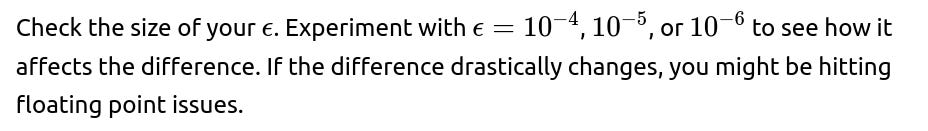
What are some potential numerical stability issues?

Floating point arithmetic can cause problems, especially when ϵϵ is very small. The finite difference approximation:

involves subtracting large numbers that might be very close in magnitude, leading to catastrophic cancellation. Sometimes you might use a slightly larger ϵ, but that might reduce the approximation’s theoretical accuracy. Another approach is to use higher precision data types (e.g., float64 instead of float32), or to carefully calibrate ϵ. Also, if your cost function saturates or is extremely large, it might hamper the reliability of your gradient checks.

How do you interpret differences between the numerical and backprop gradients?

The typical measure is the relative error:

Is gradient checking feasible for large neural networks?

Directly applying gradient checking to every single parameter in a large network is computationally expensive. If your model has millions of parameters, numerically checking each parameter with ϵ-perturbations requires multiple forward passes per parameter. This is extremely costly. Instead, you can:

Check a random subset of parameters (for example 50 or 100 parameters) to get a rough idea if there is a glaring implementation issue.

Check only a small network or a smaller version of your network architecture (fewer layers or smaller dimension) to confirm that the gradient logic works. If your code is modular, the same logic typically extends to bigger networks.

Use built-in features of certain frameworks that do symbolic gradient comparisons (though that can also be complicated if you have a lot of custom ops).

What are the differences between symbolic differentiation, automatic differentiation, and numerical gradient checking?

Symbolic differentiation involves analytically computing the exact derivative expression from a symbolic math perspective, as tools like Sympy might do. This can become very complicated for large expressions, though it yields an exact formula. Automatic differentiation, used in frameworks like TensorFlow or PyTorch, systematically applies the chain rule at the computational graph level. Numerical gradient checking is a pure numerical approach that approximates the derivative.

In practice, we rely on automatic differentiation for speed and correctness. Numerical gradient checking is slower but used as a reference check to confirm the correctness of the auto-differentiated or hand-coded backprop derivatives.

How should the cost function be handled in gradient checking if it has multiple components (for example, data loss plus regularization)?

If your cost function is J(θ)=L(θ)+R(θ) (where L(θ) might be the data term and R(θ) the regularization term), then for gradient checking, you must ensure that J(θ) in your finite difference approximation includes both components—exactly the same function you differentiate in the backprop. If you only compute L(θ) numerically but your backprop includes R(θ), or vice versa, you’ll have inconsistencies. This is a common source of errors. Always ensure that the same cost function is used in both the forward pass for numerical checking and the backward pass.

Could random noise or stochastic sampling break gradient checking?

What do you do if your gradient checking fails?

If there’s a large discrepancy:

Simplify your model. Try a simpler scenario (like a single data point or a very small network) that you can manually verify to ensure that you can isolate the bug.

Compare partial derivatives dimension by dimension. Sometimes you can find a dimension (or subset of parameters) where the numerical gradient and the backprop gradient diverge a lot, and that can pinpoint exactly which part of the code is broken.

Log intermediate values. For instance, check partial sums or intermediate activations to see if there’s an obvious mismatch.

Check your backprop step by step. If your model is complex, check each layer’s forward and backward logic. If you suspect a certain custom operation, verify that partial derivative individually.

Once you fix the problem, run gradient checking again. A small threshold mismatch can often be a sign of a single missing factor or a sign mismatch. A large mismatch might be more fundamental, like forgetting part of the chain rule.

Summary of Why Gradient Checking is Important

Gradient checking provides a definitive way to confirm that the analytical gradient computation—whether done by hand-coded backprop or by a deep learning framework’s custom components—is correct. By doing a simple but computationally costly numerical approximation of the gradient, you gain confidence that you are descending in the right direction, not being misled by an arithmetic bug. This technique is not generally used during the entire training cycle but is extremely valuable for debugging and validation.

It is an indispensable tool in a serious Machine Learning job interview context because it tests your fundamental understanding of how derivatives are computed in neural networks and your ability to debug issues that might arise when building or customizing models.

If you do gradient checking carefully, watch out for numerical pitfalls, fix seeds to remove randomness, and interpret the relative difference properly, you will either verify the correctness of your implementation or locate bugs that might otherwise cause serious training failures.

Could gradient checking be used beyond neural networks?

Yes, gradient checking can be used for any model that relies on gradient-based optimization: logistic regression, support vector machines with differentiable kernels, specialized generative models, or any function you can define a cost for. As long as you have a parameter vector θ and a cost function J(θ), you can numerically compute partial derivatives to validate an analytical gradient.

Gradient checking remains a universal debugging strategy for gradient-based methods, even though it is famously taught alongside neural network backpropagation. The primary limitation is its computational expense, so it is most feasible for smaller-scale checks or partial checks on random subsets of parameters in large-scale models.

---

Below are additional follow-up questions

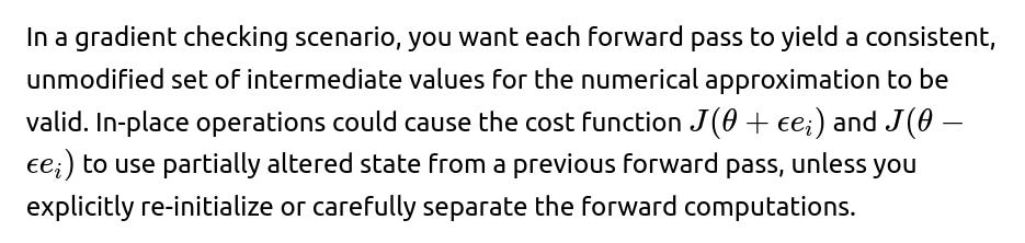
How can gradient checking be adapted when certain layers use in-place operations that might overwrite intermediate values in frameworks like PyTorch?

When a layer or function uses in-place operations (e.g., in PyTorch, something like in-place ReLU or in-place parameter modifications), the internal computational graph might be compromised because the intermediate tensors are overwritten. This can complicate or even break gradient checking and automatic differentiation if not done carefully.

Pitfalls and edge cases include:

• Forgetting to clone the parameters or certain buffers before applying the small perturbations.

• Accidentally carrying state from the previous forward pass that skews the cost computation.

• Having certain layers (like BatchNorm) track running averages in-place, which can interfere with gradient checks unless those running averages are either frozen or consistently reset.

In practice, you can avoid many issues by either disabling in-place operations or by running gradient checks in a purely functional mode (i.e., the forward pass does not modify any internal variable without making a copy first). If your framework allows it, you can also detect or disable in-place ops during debugging. For example, PyTorch can sometimes issue warnings or errors if a function modifies values needed for the backward pass. For gradient checking, an even simpler fix is to avoid in-place operations altogether while you do your debug checks, then reintroduce them later for performance benefits.

What challenges arise if the cost function is piecewise or not differentiable at certain points?

In many deep learning architectures, you might have non-smooth operations: for example, ReLU units (max⁡(0,x)), absolute value operations, or custom piecewise functions. These can produce kinks or corners where the derivative is undefined or discontinuous. Gradient-based methods in frameworks like PyTorch or TensorFlow typically handle this by defining subgradients or adopting a particular convention at non-differentiable points.

Pitfalls to consider:

• If your cost function has a large set of non-differentiable points (e.g., L1 regularization with ∣w∣ terms), you might see very erratic or large gradient-checking errors for parameters that cross zero.

• Sometimes frameworks define a subgradient for non-differentiable points, but your numerical difference might not match that convention exactly.

• A small ϵ can cause numerical instability near corners, while a larger ϵ might yield a smoothed-out approximation that doesn’t capture the correct subgradient behavior.

To handle these scenarios, you can:

• Check if your framework’s subgradient definition matches your numerical approach, acknowledging that exact matches at corners might be impossible.

• Evaluate your gradient checks at parameters away from the boundaries or test them across multiple random seeds so that you don’t repeatedly land on non-differentiable points.

• Temporarily replace the non-smooth operation with a smooth approximation (e.g., Softplus instead of ReLU) just for gradient checking, to see if the rest of your backprop pipeline is correct.

How would gradient checking be affected if the network includes random data augmentation steps in the forward pass?

Potential pitfalls include:

• Believing the gradient check is failing when, in reality, it is just seeing different augmented versions of the data.

• Attempting to lower ϵ or tweak other parameters without realizing that the fundamental issue is the randomness in the forward pass.

To handle it properly:

What happens if different components of the model’s output share parameters and you want to check gradients for each output dimension separately?

In multi-output models, you might define a cost function J(θ) that is itself a combination of separate losses (one per output dimension). For example, in multi-task learning, you might sum or weight the losses for each task. If a single parameter vector θ is shared across tasks or across multiple outputs, you need to confirm that your gradient calculation includes all partial derivatives from each output dimension’s contribution.

Key considerations:

• If you decide to do partial gradient checks for each sub-loss separately, you must isolate the cost function to that sub-loss in both the numerical and analytical passes. Alternatively, you can define the total cost as the sum of sub-losses, then do gradient checking on the total cost. The important point is consistency.

Edge cases:

• Some outputs might not depend on all parameters, resulting in zero partial derivatives. If you see spurious non-zero values in your backprop, that suggests a bug.

• In some frameworks, you might forget to zero out the gradients for each backward pass, causing the gradient from one output dimension to “leak” into the gradient check for another dimension.

How do you perform gradient checking if the network is large and distributed across multiple GPUs or machines?

When a model is large enough to require distributed training, the computational graph and parameters are split across multiple GPUs or nodes. Gradient checking in this setting can become complex because:

• Each forward pass might require synchronization across multiple devices or processes. Perturbing a parameter on one GPU might require transferring updated values and ensuring consistency on all devices.

• Communication overhead can become a bottleneck, as you need multiple forward passes per parameter (or at least per parameter subset).

• You have to confirm that the same mini-batch or data partition is used consistently in each forward pass; distributed data parallel setups often split the data across workers.

Possible strategies:

• Perform gradient checking in a single-machine or single-GPU environment with a smaller model slice or a toy setup. If that slice passes gradient checks, you can be more confident in the overall correctness once you scale up.

• Randomly sample a subset of parameters that reside across different devices, checking only those. This partial check can still catch many implementation bugs.

• Ensure your distributed training code path does not introduce additional randomness or data shuffling across nodes that invalidates the comparison.

Pitfalls:

• Overlooking synchronization barriers: if you perturb a parameter but the rest of the system is using stale or unperturbed parameters, you can get inconsistent cost measurements.

• Communication libraries might have precision differences in the data (e.g., automatic downcasting to FP16 or BF16). This can lead to a mismatch in numerical vs. analytical gradients if not accounted for.

How can we handle gradient checking in real-time or streaming applications where data might be arriving continuously?

Certain machine learning systems operate on streaming data (e.g., real-time recommendation engines) and update parameters incrementally. In this context, gradient checking is not as straightforward because at the exact moment you perturb a parameter, the underlying data distribution could shift or the next batch might differ entirely.

Potential pitfalls:

• The system might revert parameters or incorporate partial updates in between your finite difference evaluations, making the forward passes inconsistent.

Practical approaches:

• Save snapshots of the system state so you can revert to the exact same system state before each forward pass. This might be computationally expensive, so typically you only do it for a smaller scale or for debugging.

Could we use higher-order methods (like the Hessian or second-order checks) to verify correctness beyond just the first derivative?

In principle, yes. You could verify second-order derivatives (the Hessian matrix) by using finite differences of finite differences, or by comparing them with automatic differentiation methods that compute Hessians. This can be useful in advanced optimization methods (e.g., natural gradient or Newton-type methods) that rely on second-order information.

However, second-order checks magnify the cost:

• You already need multiple function evaluations for each parameter dimension to do first-order gradient checks. For second-order checks, you might need an even larger number of function evaluations per pair of dimensions.

• Numerical error can accumulate even more for higher-order derivatives, making it trickier to interpret discrepancies.

Edge cases:

• Many neural networks use piecewise linear or non-smooth activations, so the Hessian might be undefined or zero in large regions. This can make second-order checks less informative for ReLU-based networks.

• In large-scale practical systems, second-order checks are rarely done except in specialized research contexts. When done, one might only check a small subspace of parameters or rely on approximations like the generalized Gauss-Newton matrix.

How do you interpret gradient checking in the presence of quantized or mixed precision training?

With the rise of GPU accelerators that use half-precision (FP16) or bfloat16 for faster computation, gradients might be stored in lower precision than float32. Numerical gradient checking typically relies on float64 or at least float32 arithmetic to get stable finite difference approximations.

Potential pitfalls:

• Rounding errors can be larger in half precision, so you might see bigger discrepancies between numerical and backprop gradients than you would in full precision.

A common workaround is to do gradient checking in full precision using a smaller version of your model or by temporarily disabling mixed precision. Once verified, you re-enable mixed precision for performance in actual training.

How can subtle indexing errors in custom layers manifest during gradient checking?

One of the most common real-world issues in implementing new layers or modules is indexing errors. For instance, suppose you wrote a custom embedding layer or a custom attention mechanism where you manually slice or gather elements from a tensor. If your slicing logic is off by one index or you accidentally sum across the wrong dimension, you might produce partial derivatives that deviate in a subtle way.

Potential consequences:

• The cost might still decrease slowly in normal training, giving you a false sense of correctness. However, the discrepancy in gradient checking (especially dimension by dimension) would catch the mismatch.

• If the bug is only triggered for certain slices of the data (like boundary indices in an embedding table), a random gradient check might not catch it. You might have to systematically test specific parameter indices that correspond to the edge cases.

To mitigate this risk:

• Write unit tests or smaller sub-tests for the custom layer in isolation, verifying forward/backward correctness on artificially small input shapes (like a single sample) so you can more easily trace the computations.

How do you handle gradient checking in modular or library code where you don’t have full access to the internal computations?

In large teams or codebases, you might import a library (say, for a particular layer or data processing module) where you can’t directly modify the forward pass to do gradient checking. Alternatively, the library might rely on heavily optimized GPU code or vendor-proprietary kernels.

In these scenarios:

• Try to confirm whether the library includes an option to enable or debug gradients. Some libraries have built-in checks or reference implementations in pure Python you can switch on for verification.

• If you can’t alter the library, you might only be able to check the overall end-to-end gradient from your entire pipeline. If the library is correct, it should pass, but if you see a mismatch, diagnosing the root cause might be difficult without internal checks.

• Another option is to replicate the library’s behavior in a simplified or partial form in Python (or any accessible language) and do gradient checking there. You can compare the library’s outputs with your reference implementation. This approach is more time-consuming but can be the only way to isolate bugs in black-box or closed-source components.

Edge case:

• Some libraries implement approximate algorithms (like sampling-based approximations or Monte Carlo estimation). In that case, the same data or random seed must be used to match the library’s result for each forward pass, else your gradient check might register large divergences due to differences in sampling.