ML Interview Q Series: Essential Metrics for Evaluating Fraud Detection Binary Classifiers

📚 Browse the full ML Interview series here.

Say you need to produce a binary classifier for fraud detection. What metrics would you look at, how is each defined, and what is the interpretation of each one?

This problem was asked by Uber.

You typically examine multiple metrics beyond raw accuracy because fraud detection tasks often involve highly imbalanced data. Each metric offers a different perspective on how well your classifier is performing. Below are the major metrics and their interpretations.

Accuracy

Accuracy is the fraction of predictions your model gets right out of the total number of predictions made. If you have a confusion matrix:

where TN is the number of true negatives, FP is the number of false positives, FN is the number of false negatives, and TP is the number of true positives, then Accuracy can be expressed as

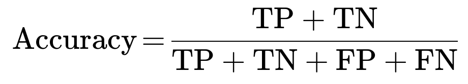
In fraud detection, accuracy by itself can be misleading when the majority of transactions are non-fraudulent (negative class). If 99% of transactions are legitimate, a naive classifier that always predicts “legitimate” would achieve about 99% accuracy but be useless at detecting fraud.

Interpretation for Fraud Detection

High accuracy does not necessarily mean the model catches fraud. You might be correct on most legitimate transactions but miss the rare fraudulent ones. Accuracy is generally not the sole metric used in scenarios where the class distribution is skewed or the cost of certain misclassifications is very high.

Precision

Precision (also called Positive Predictive Value) measures among all transactions predicted as “fraud,” how many actually were fraudulent. It is defined as:

Interpretation for Fraud Detection

High precision means that when your model flags a transaction as fraud, it is very likely to be correct. This is often critical for scenarios in which false positives are costly, such as when investigating a transaction flagged as fraudulent requires significant resources. If precision is too low, you waste time and money investigating transactions that turn out not to be fraud.

Increasing precision might reduce the recall (we discuss recall below) because you become more conservative about labeling anything as fraud. A high-precision, low-recall classifier would rarely be wrong in its fraud prediction but might miss many fraudulent transactions altogether.

Recall (Sensitivity, True Positive Rate)

Recall indicates among all actual frauds, how many your model identified. It is defined as:

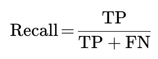
Interpretation for Fraud Detection

High recall means that your model catches most fraudulent transactions. A low recall is dangerous because it means a large fraction of fraud goes undetected. However, pushing recall higher often increases false positives, which in turn lowers precision.

In fraud detection, you usually prefer to err on the side of recall, especially if the cost of missing fraud (false negatives) is substantial. Balancing the trade-off between recall and precision is one of the main tasks in dealing with imbalanced classification problems.

F1 Score

F1 Score is the harmonic mean of precision and recall:

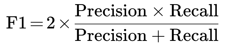
Interpretation for Fraud Detection

An F1 Score balances precision and recall into a single metric. It is especially useful if you need a single statistic that accounts for both. A high F1 means both precision and recall are reasonably high. However, by collapsing two metrics into one, you might lose information about the specific trade-off between catching fraud (recall) and minimizing false alarms (precision). Still, F1 is a common choice in heavily imbalanced settings where accuracy is not informative.

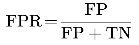
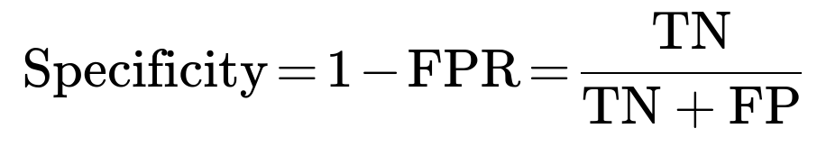
False Positive Rate (FPR) and True Negative Rate (Specificity)

False Positive Rate is the fraction of legitimate transactions that were incorrectly classified as fraud out of all legitimate transactions. It is given by:

The complement of FPR is the True Negative Rate (Specificity), which is:

Interpretation for Fraud Detection

False Positive Rate is critical because a high number of false positives means many legitimate transactions are flagged. This could lead to unnecessary customer friction. Specificity measures how good you are at identifying legitimate transactions as legitimate. In a balanced or small-scale classification, you may not focus on specificity, but for large-scale fraud detection, it matters because you don’t want to annoy a massive number of non-fraudulent customers with false alarms.

ROC Curve and AUC (Area Under the Curve)

An ROC curve plots the True Positive Rate versus the False Positive Rate as you vary the classification threshold. The AUC (Area Under the Curve) summarizes the entire ROC curve into one number that ranges from 0.5 (no better than random guessing) to 1.0 (perfect classification).

Interpretation for Fraud Detection

AUC-ROC helps you see how well your classifier can rank fraud cases as more suspicious than non-fraud. It also provides a threshold-independent view of performance. However, in highly imbalanced problems, the ROC curve can sometimes be overly optimistic because a large number of negatives can make your FPR look artificially small. Often in fraud detection, you might prefer the Precision-Recall AUC as well.

Precision-Recall Curve and Average Precision

A Precision-Recall (PR) curve shows the trade-off between precision and recall as you change the classification threshold. Average Precision (AP) is the area under the precision-recall curve.

Interpretation for Fraud Detection

The PR curve (and the corresponding average precision metric) is often more telling for heavily imbalanced data because it focuses on performance in predicting the minority (fraud) class. If your PR curve remains high (both in terms of precision and recall) at varying thresholds, it means your classifier is consistently good at identifying fraud while minimizing false alarms.

When to Use Each Metric

Different stakeholders may value different metrics. Fraud detection systems usually emphasize precision if the cost of investigating false positives is extremely high, or emphasize recall if missing a fraudulent transaction is more damaging. Threshold tuning is a central strategy: you can shift the threshold to favor a higher recall (catching more fraud) at the expense of precision, or vice versa.

Models often need to meet a certain threshold of recall (to catch enough fraud) while also preserving a reasonable precision level (to manage operational costs). You typically look at a combination of:

Accuracy (as a quick sanity check) Precision, Recall, F1 ROC AUC and/or Precision-Recall AUC False Positive Rate and Specificity, for operational considerations

In real-world fraud detection, you also consider business-driven cost matrices that weight the relative costs of different types of errors. This might lead you to prioritize certain metrics (e.g., recall over precision) or define custom metrics tailored to business constraints.

Below are some illustrative code snippets in Python to compute these metrics. Assume we have true labels y_true and predicted labels y_pred:

from sklearn.metrics import confusion_matrix, accuracy_score, precision_score, recall_score, f1_score, roc_auc_score, average_precision_score

cm = confusion_matrix(y_true, y_pred)
tn, fp, fn, tp = cm.ravel()

accuracy = accuracy_score(y_true, y_pred)
precision = precision_score(y_true, y_pred)
recall = recall_score(y_true, y_pred)
f1 = f1_score(y_true, y_pred)
roc_auc = roc_auc_score(y_true, y_pred)  # Might require predicted probabilities or decision_function
avg_precision = average_precision_score(y_true, y_pred)  # Also typically computed on probabilities

print("Confusion Matrix:", cm)
print("Accuracy:", accuracy)
print("Precision:", precision)
print("Recall:", recall)
print("F1 Score:", f1)
print("ROC AUC:", roc_auc)
print("Average Precision:", avg_precision)

When evaluating a fraud detection classifier, you typically generate predictions in probability form and then sweep different thresholds to plot the ROC curve or PR curve and analyze the trade-offs thoroughly.

What are potential pitfalls of relying on accuracy alone in a fraud detection scenario?

Because the fraud class is rare (often less than 1% of transactions), a model that predicts every transaction as “legitimate” can achieve extremely high accuracy simply by following the majority class. However, such a model is effectively useless because it does nothing to catch fraud. Relying solely on accuracy fails to capture how well the model handles the minority class. You might overlook crucial signals in the data if you focus on this simplistic metric. Furthermore, organizationally, focusing on accuracy might lead to under-investment in a model’s ability to catch rare but costly fraudulent cases.

How would you choose the threshold for deciding if a transaction is fraud or not?

Threshold tuning typically involves adjusting the probability cutoff at which a transaction is labeled as fraudulent vs. legitimate. You often start with a default threshold of 0.5, but you tune this based on the business trade-offs. If missing a fraudulent transaction (false negative) is very costly, you lower the threshold to increase recall (while likely reducing precision). If investigating a false alarm (false positive) is extremely expensive or causes negative customer experience, you raise the threshold to improve precision (while lowering recall).

You might use the Precision-Recall curve or the ROC curve to find an optimal operating point. In practice, you could use a cost function or a cost matrix that translates false negatives and false positives into monetary or other business impacts. You then pick the threshold that optimizes that cost function. A typical approach includes cross-validation on a training set to find the threshold that best meets your performance and cost objectives, and then locking down that threshold for the production environment.

Why might the Precision-Recall AUC sometimes be more informative than the ROC AUC?

In an extremely imbalanced classification scenario, the ROC curve can give a misleadingly optimistic view of performance because the large number of true negatives (the legitimate class) can keep the false positive rate (FPR) low even when you are not doing a good job in identifying the minority (fraud) class. The Precision-Recall curve explicitly focuses on how well you detect the minority class and how reliable those predictions are. The area under the PR curve (average precision) can thus be a clearer indicator of how well your model detects fraud at various thresholds.

In a scenario where fraud is extremely rare, a small shift in the number of false positives or false negatives can drastically change the practical business impact. Precision and recall directly reflect these minority class outcomes, making Precision-Recall AUC often more relevant for real-world fraud detection systems.

If you had to pick only one metric, which would it be and why?

Different businesses have different priorities, so the “best” single metric can vary. In many fraud detection settings, recall is critical because missing a fraudulent transaction can have significant costs. However, focusing only on recall can overwhelm you with false positives. Some organizations might still insist on a minimum precision to keep false alarms manageable.

In practice, a combined metric like F1 or the average precision (area under the PR curve) is often chosen to balance these considerations if forced to rely on a single scalar. Still, it is almost always better to monitor at least two metrics simultaneously (e.g., track precision and recall together) or to define a custom cost-based metric that incorporates actual business impacts of each error type.

What are other subtle issues or real-world considerations when applying these metrics in production?

Model drift occurs when fraud patterns change over time. Your model might see reduced recall or precision if the criminals adopt new tactics. Monitoring the metrics over time is necessary to catch drift early.

Data leakage can happen if some features unintentionally encode future knowledge about the transaction outcome. This leads to overly optimistic metrics during training but poor performance in production.

Thresholds might need dynamic adjustments. If fraud patterns spike during certain times of year (e.g., holiday seasons), you might adjust thresholds or model strategies dynamically.

Class imbalance can shift over time. As the ratio of fraudulent to legitimate transactions changes, previously determined thresholds might become suboptimal.

Cost-sensitive learning or custom cost functions are often used in real production systems. You might incorporate investigation costs, reputational risks, or chargeback amounts into the metric so that each TP, FP, TN, and FN is translated into a more tangible cost.

Human-in-the-loop systems are often used. You might have a model that flags suspicious transactions, and then an analyst manually reviews them. This process leads to more complexity in defining “success.” It might be acceptable to have more false positives if the manual review process is quick and less costly.

Could you show how to compute these metrics for a fraud dataset that is highly imbalanced?

Below is a short Python example. Assume you have a dataset with significantly more legitimate transactions than fraudulent ones. The code is not using bullet points but shows a typical approach:

import numpy as np
from sklearn.model_selection import train_test_split
from sklearn.ensemble import RandomForestClassifier
from sklearn.metrics import confusion_matrix, classification_report

# Suppose X contains our transaction features and y contains 0 for legitimate and 1 for fraud
X = ...
y = ...

X_train, X_test, y_train, y_test = train_test_split(X, y, stratify=y, test_size=0.2, random_state=42)
model = RandomForestClassifier(n_estimators=100, random_state=42)
model.fit(X_train, y_train)

y_pred = model.predict(X_test)
cm = confusion_matrix(y_test, y_pred)
report = classification_report(y_test, y_pred)

print("Confusion Matrix:")
print(cm)
print("Classification Report:")
print(report)

The confusion matrix shows the count of TN, FP, FN, and TP. The classification_report includes precision, recall, and F1 Score for each class as well as macro/micro averages. For deeper analysis, you typically compute ROC AUC or Precision-Recall AUC using the model’s predicted probabilities:

from sklearn.metrics import roc_auc_score, average_precision_score

y_scores = model.predict_proba(X_test)[:, 1]
roc_auc = roc_auc_score(y_test, y_scores)
avg_precision = average_precision_score(y_test, y_scores)

print("ROC AUC:", roc_auc)
print("Average Precision (PR AUC):", avg_precision)

You then analyze these values with respect to the cost matrix or the current operating constraints. You might choose a threshold for y_scores other than 0.5 if your goal is higher recall or higher precision.

How might a cost matrix shape the choice of metric?

A cost matrix translates each type of classification outcome into a monetary or organizational impact. For example, let:

Cost(False Negative) = $1000 Cost(False Positive) = $50 Cost(True Positive) = -$1000 (you save this amount, or recover it) Cost(True Negative) = -$1 (small resources spent but no big negative)

You would then compute a cost-based metric:

Minimizing total cost (or maximizing negative cost) can lead you to a threshold or model strategy quite different from the one that maximizes F1 or accuracy. This approach is often more aligned with real-world objectives, especially in fraud detection, where the cost of missing a fraud (a false negative) is frequently much larger than a false positive. Incorporating these real-world costs is essential for a well-tuned fraud detection system.

If a model shows high recall but poor precision, what are some strategies to improve it?

Collect more representative data. The low precision might come from limited fraudulent examples, so more data (or targeted data enrichment) can help.

Engineer features that better separate fraudulent from legitimate transactions. Good features help reduce overlap between the classes.

Apply undersampling or oversampling techniques (or specialized approaches like SMOTE) to improve how the training process handles imbalance. However, be careful with how sampling might shift the distribution.

Use models or ensembling techniques that handle imbalanced data more effectively, such as XGBoost or LightGBM with custom objective functions or class-weight adjustments.

Tweak the decision threshold. Even a high-recall, low-precision model might find a better balance with a more optimal threshold. You can do a grid search over thresholds and measure how precision, recall, and cost-based metrics change.

Filter out easily flagged legitimate transactions (i.e., transactions that are obviously non-fraud) first in a quick pre-check stage, so your main classifier can focus on more ambiguous transactions. This can effectively reduce the class imbalance in the second-stage classifier.

How do you handle changes in fraud behavior over time (concept drift)?

Continuously monitor the model’s performance metrics, especially recall and precision, to detect a shift in data distributions or fraud patterns.

Retrain the model on the most recent data that reflects emerging fraud tactics. This can be done incrementally or periodically (e.g., retraining every day/week/month depending on transaction volume and drift speed).

Use adaptive or online learning algorithms that can update their parameters in real-time as new data comes in.

Maintain a feedback loop. Fraud investigators or customers themselves (through chargeback claims or dispute processes) provide ongoing labels for flagged transactions. These feedback labels help you keep the training data up to date.

Regularly evaluate the model with backtesting. Partition historical data into time-based windows to simulate how the model would have performed when facing older distributions vs. new patterns.

How would you explain these metrics to a non-technical stakeholder?

Accuracy is how many transactions you classify correctly overall, but it can be misleading when fraud is rare. Precision is how reliable the “fraud” label is. Recall is how many frauds you actually catch. F1 combines precision and recall into one measure. In a highly imbalanced domain like fraud detection, you need to look at more than just accuracy because missing a small fraction of transactions can mean a big financial loss.

For a business stakeholder, focusing on cost or monetary impact is often best. Show how different thresholds would influence the number of false alarms vs. missed fraud, and how that translates into dollars lost or spent.

How does real-time fraud detection affect metric computation?

In real-time fraud detection, you typically have to make immediate decisions. This means delayed or second-stage investigations might still refine your final label, and you might initially only have partial data. Online evaluation methods become important because you need to track metrics continuously.

When you flag a transaction as fraud in real-time and a manual investigation confirms or refutes it, you update your metrics. This might include building a rolling confusion matrix or a rolling average of precision and recall. The challenge is that the label for a flagged transaction might come hours or days later. Handling that label delay is a key design consideration in real-time detection systems.

How would these metrics apply if the definition of “fraud” is subjective?

In some domains, “fraud” can be ambiguous and subject to interpretation, especially if it depends on whether a user claims a dispute or a bank refunds a charge. The ground truth label might be noisy or incomplete. In that scenario, the confusion matrix might not fully reflect the actual reality of fraud.

Strategies include building consensus labels from multiple data points or multiple reviewers, assigning confidence levels to each label, or structuring the dataset to separate “confirmed fraud” from “suspected fraud.” You might also use semi-supervised methods if you have partially labeled data. But your evaluation metrics could be less definitive due to uncertain or subjective ground truth.

How would you apply different metrics over different subsets of data?

It is common to segment data by transaction type, region, or risk category. For instance, transactions above a certain amount might warrant a stricter threshold. You could measure precision and recall specifically in high-risk subsets. That granular approach often reveals that a single global threshold might not be optimal across all transaction types.

You might have one threshold or even a different model for high-risk transactions, where you heavily favor recall, and a more balanced model or threshold for low-risk transactions. Monitoring metrics at these subgroup levels ensures you do not overfit to one particular segment while ignoring important variations in the data.

Below are additional follow-up questions

How do you ensure that the model’s output probabilities are well-calibrated, and why does calibration matter in fraud detection?

Calibration is about making sure the predicted probabilities align with actual empirical probabilities. For instance, if a model outputs a probability of “fraud” equal to 0.8 for 100 transactions, ideally around 80 of them would indeed be fraudulent in reality. In many machine learning models, especially those that optimize primarily for classification accuracy or similar metrics, the raw probabilities might not reflect the true underlying likelihood of fraud. This misalignment can lead to suboptimal threshold-setting, cost estimates, and risk management decisions.

Calibration in Practice

One common approach is Platt scaling, where you train a separate logistic regression model on the model’s raw outputs to map them to well-calibrated probabilities. Another is isotonic regression, a non-parametric method that can flexibly map raw scores to probabilities.

Potential Edge Cases

A potential pitfall is when your training set for the calibration method does not reflect the full distribution of actual transactions—especially if fraud patterns change or the dataset is unbalanced in a new way. If the calibration set is not updated regularly, or if it excludes certain rare but important scenarios (e.g., large transfers, overseas transactions), the calibrated probabilities might still be skewed. Another subtlety is that even if the model’s overall calibration looks good on average, there may be specific ranges or subpopulations where the calibration is poor (e.g., transactions below a certain value might be overestimated in fraud probability).

Value of Good Calibration

Well-calibrated probabilities allow risk analysts to more accurately estimate expected losses or returns. In fraud detection, having reliable confidence estimates helps you to set dynamic decision thresholds: for example, investigating transactions predicted at 0.90 or higher probability. If the probabilities are not well-calibrated, you may either waste resources investigating transactions that are less likely to be fraud than predicted or miss out on catching fraudulent transactions because you are too lenient.

Implementation

Below is a simplified code example in Python to illustrate the calibration process with isotonic regression:

from sklearn.model_selection import train_test_split
from sklearn.ensemble import RandomForestClassifier
from sklearn.calibration import CalibratedClassifierCV, calibration_curve
import numpy as np

# Suppose we have X, y (0 = legit, 1 = fraud)
X_train, X_val, y_train, y_val = train_test_split(X, y, stratify=y, test_size=0.2)
base_model = RandomForestClassifier(n_estimators=100)
base_model.fit(X_train, y_train)

# Calibrate the model using isotonic
calibrated_model = CalibratedClassifierCV(base_estimator=base_model, method='isotonic', cv='prefit')
calibrated_model.fit(X_val, y_val)

# Evaluate calibration
prob_true, prob_pred = calibration_curve(y_val, calibrated_model.predict_proba(X_val)[:,1], n_bins=10)

Analyzing the calibration curve (comparing “prob_true” vs. “prob_pred”) reveals how closely predicted probabilities match the fraction of positive cases. Good calibration ensures you can trust the probability outputs in real-world decisions.

What if the fraud detection dataset is extremely large? How would you scale the training and evaluation of these metrics?

When dealing with extremely large datasets—potentially millions or even billions of transactions—computational efficiency and distributed processing become vital. Traditional single-machine methods can be prohibitively slow or run out of memory.

Strategies for Large-Scale Data

1. Distributed Computing Frameworks Using Spark, Hadoop, or other distributed frameworks can parallelize data preprocessing, model training (when supported), and metric computation. Libraries like MLlib in Apache Spark or TensorFlow Distributed can handle large-scale training more efficiently.

2. Incremental / Online Learning With online learning algorithms such as stochastic gradient descent (SGD) or certain implementations of random forests, you can stream data in mini-batches and update model parameters iteratively. This approach is helpful if the data arrives in real time or is too large to process all at once.

3. Subsampling and Stratification Because fraud is a rare event, you might stratify and sample your data to keep it manageable. If you have 100 million legitimate transactions and 1 million fraudulent ones, you could take a random subset of legitimate transactions (say, 10 million) and all fraudulent ones to train your model. You still capture enough legitimate variety while speeding up training. However, you must be careful with how you sample so as not to lose important patterns, especially borderline legitimate transactions that look similar to fraud.

Potential Pitfalls

A major pitfall is sample bias: if the data is not carefully stratified or if certain transaction types get disproportionately removed, your model can become poorly calibrated or biased against certain subgroups. Another edge case is when computations like metrics or calibration curves become intractable at scale, pushing you to rely on approximate methods (e.g., sampling at evaluation time).

Monitoring Metrics at Scale

Instead of computing metrics on every single transaction, you could track them on large but manageable batches (e.g., monthly or weekly slices). You might also implement streaming metrics that update incrementally as new data arrives.

How do you handle delayed ground truth labels in fraud detection, and how does it affect metric computation?

Delayed Labels Scenario

In many fraud detection systems, you only learn that a transaction was fraudulent days, weeks, or even months later—often due to manual investigations, chargebacks, or dispute resolutions. This delay means that at the time you score a transaction, you do not immediately know whether your prediction was correct.

Approaches to Address Delayed Labels

1. Holdout Period You maintain a “holdout period” of data for evaluation where enough time has passed to confirm the final fraud/legitimate label. This ensures your evaluation metrics reflect real outcomes.

2. “Label-Lag” Correction You might store predictions alongside transactions, then periodically update the confusion matrix once labels become available. This implies your real-time metrics might undercount actual fraud until it’s confirmed.

3. Proxy Labels Some businesses use proxy signals (e.g., a transaction that triggers certain risk signals or user complaints within a short window) as an interim label, though this can introduce noise. Over-reliance on proxy labels can distort your metrics, causing you to overestimate or underestimate true performance.

Pitfalls and Edge Cases

One subtlety is that a large fraction of fraudulent transactions might not even be labeled if there’s no formal dispute mechanism. Another edge case arises if disputes can be fraudulent themselves (e.g., “friendly fraud,” where a legitimate customer falsely claims a transaction was fraudulent to receive a chargeback). This further complicates the ground truth. To mitigate these pitfalls, many fraud teams invest in specialized label-collection pipelines and cross-reference multiple data sources (e.g., chargeback data plus internal investigations plus confirmations from other financial institutions).

How does seasonality or periodic changes in behavior affect your choice of metrics and overall fraud detection strategy?

Seasonality in Fraud Patterns

Fraud can spike around specific times, such as holidays or major sales events. Legitimate transaction volumes also increase during certain periods, potentially shifting the ratio of fraud to legitimate transactions.

Metric Stability Over Time

If you evaluate your model at a single point in time (or on an aggregated dataset) without considering temporal splits, you might not see how recall and precision vary month-to-month. You could be underprepared for seasonal anomalies, leading to a spike in false negatives or false positives during peak periods.

Practical Approaches

1. Rolling Window Evaluation You can maintain a rolling (or sliding) window—e.g., using the most recent 30 days of data—to continuously measure precision, recall, F1, etc. This ensures you detect performance degradation promptly.

2. Multiple Thresholds per Season Some organizations define different classification thresholds for different seasons. For example, around the holiday season, you might lower your threshold to be more aggressive in catching fraud (boosting recall) because fraud attempts historically increase, while in quieter periods, you might set a higher threshold to reduce false positives.

3. Ensemble Models Across Seasons You could train season-specific models or an ensemble of models that handle different transaction volumes and patterns. However, be mindful of complexity and operational overhead. Also, ensure that your evaluation strategy covers each seasonal pattern properly.

Edge Cases

A subtle pitfall is that seasonality can change year to year—fraudsters adapt. If you rely on last year’s holiday fraud patterns to set thresholds for this year, that may be outdated. Another potential issue is “concept drift,” where fraud tactics evolve, making historical data less predictive of future fraud, even for the same seasonal period.

How do you address interpretability or explainability of your fraud detection metrics and model decisions?

Importance of Interpretability

Fraud detection decisions can have significant repercussions for customers (e.g., blocking a legitimate payment or freezing an account). Many financial regulations also demand some level of transparency. Thus, interpretability matters not just at the model level, but also at the metrics level. Stakeholders want to understand how well the model performs and why certain metrics are chosen.

Metrics Explanation

When explaining metrics like precision or recall to a non-technical stakeholder, you should connect them to business outcomes. For instance, “A recall of 95% means we’re catching nearly all fraudulent transactions, but you can expect about 5% to slip by,” or “We have a precision of 80%, so 20% of the transactions we flag turn out to be false alarms.”

Model Interpretability Techniques

1. Feature Importance Techniques like SHAP (SHapley Additive exPlanations) or LIME (Local Interpretable Model-agnostic Explanations) can help identify which features most influence a fraud prediction. This is crucial when regulators or internal audit teams ask, “Why was this transaction flagged?”

2. Surrogate Models You might use a simpler model (e.g., a decision tree) as a surrogate to approximate the predictions of a more complex model (like a deep neural network), providing a more interpretable structure for explaining the model’s overall logic.

3. Rule-Based Overlays Some organizations maintain a set of explicit rules or triggers (e.g., “Transactions above $10,000 from a new user are automatically flagged”) alongside a machine learning model. The model picks up the nuanced patterns, while the rules remain interpretable to auditors.

Pitfalls

A big pitfall is over-simplification: insisting on interpretability might lead you to deploy a less accurate model. Another edge case arises when a model is globally interpretable (overall feature importances are stable), but local decisions (for a single transaction) are still opaque due to complex interactions among features.

How can you use multi-stage (or cascading) classification to improve fraud detection metrics?

Two-Stage Classification Approach

In many production systems, you might use a lower-threshold classifier for the first pass to ensure high recall. Then, you feed only the flagged transactions into a second-stage classifier or manual review process that focuses on improving precision. Essentially, the second stage tries to filter out false positives among a smaller pool of suspicious transactions.

Benefits for Metrics

By design, the two-stage approach boosts overall recall (because the first stage is lenient and rarely misses fraud). The second stage helps improve precision (by carefully scrutinizing questionable cases). This can yield higher F1 scores while maintaining an acceptable false positive rate.

Implementation Detail

Stage 1 might be a fast or lightweight model (like a logistic regression or a simplified set of rules) that ensures real-time detection at scale. Stage 2 might be more computationally expensive (like a large gradient boosting model or a deep neural network) or even a human analyst review.

Pitfalls

1. Data Distribution Shift In the second stage, the transactions you see are not representative of the overall distribution—they’re already “suspect.” So if you train your second-stage model on these data, it might be biased or incorrectly calibrated when generalized back to the entire population.

2. Overreliance on Stage 2 You still need to ensure Stage 1 is accurate enough that you don’t flood Stage 2 with too many false positives, which would overwhelm investigators or computational resources.

3. Delay in Labeling Because Stage 2 might involve manual review, the label for those transactions can be delayed, affecting how quickly your system can learn from new fraud trends.

How do you leverage unsupervised methods or anomaly detection for potential fraud, and how do you measure success then?

Unsupervised Fraud Detection

Unsupervised or semi-supervised techniques (like autoencoders, isolation forests, or density-based methods) can detect unusual patterns without explicit fraud labels. This can be especially helpful for new types of fraud that your model has not seen.

Key Challenge in Metrics

With unsupervised methods, you typically lack ground truth labels for training. When you do eventually label some flagged transactions, you can compute metrics like precision at kk (where kk is the number of top anomalies flagged) or recall at kk. Alternatively, you can do random sampling of unflagged transactions to estimate false positives.

Interpretation Pitfalls

1. High False Alarm Rate Unsupervised anomaly detectors can be prone to flagging rare but legitimate behavior as fraud. If you rely on these flags directly in production, you may trigger high false positives and degrade user experience.

2. Domain Knowledge Integration Without domain knowledge or known fraud examples, the anomaly detector might focus on harmless outliers (like a legitimate VIP customer with unusual spending). Combining unsupervised methods with even a few labeled examples can drastically improve performance.

3. Ongoing Evaluation You must have a strategy to confirm or refute anomalies. If you don’t eventually get labels on anomalies, you can’t fully assess your recall. As a workaround, companies often route unsupervised flags to investigators, collecting labels from manual reviews.

How do you evaluate the stability of these metrics if your fraud detection model updates frequently (e.g., every hour or every day)?

Frequent Model Retraining

In high-volume fraud scenarios, you might have a pipeline that retrains your model daily or even hourly with fresh data. While this helps you adapt quickly to new patterns, it can cause fluctuations in precision, recall, and other metrics.

Approaches to Monitor Stability

1. Rolling Metrics You can maintain a rolling average of precision, recall, or F1 over a fixed time window to smooth out short-term variability.

2. Statistical Tests You can run statistical significance tests on the difference in metric values between model versions. For example, if your new model’s F1 is 2% higher but not statistically significant, you might hold off on deployment to avoid frequent model churn.

3. Canary or Shadow Deployment Before a full rollout, you can do a canary release: deploy the new model to a small fraction of traffic and compare metrics side-by-side with the existing model. This helps you detect major drops in performance or unexpected side effects.

Pitfalls

One risk is that your data pipeline might not be stable. If data ingestion changes or a new type of transaction code is introduced, your metrics could shift abruptly due to data issues rather than genuine model improvement or degradation. Another subtlety is that frequent retraining can amplify overfitting if you overreact to temporary spikes in fraud patterns. A potential edge case is if the real distribution changes so rapidly (e.g., an organized fraud ring is active for a few hours then disappears) that your weekly metrics look fine, but in practice, you missed a crucial short-lived event.

How do you measure the performance of your model in the presence of a highly dynamic fraudster adversary?

Adversarial Nature of Fraud

Fraudsters often test small transactions first to probe your detection system. Once they find a weak spot, they scale up rapidly. This means your data distribution can exhibit sudden shifts that do not follow normal concept drift patterns.

Adaptive Metrics

1. Short-Interval Evaluation Evaluate your precision and recall on daily or even hourly batches, especially focusing on newly emerging transaction patterns.

2. Weighted Metrics for Novelty You might assign extra weight or vigilance to new user accounts or IP addresses. Your metrics should reflect how well you handle these novel patterns. If you track recall only on “known” patterns but not on new or evolving patterns, you might have a false sense of security.

3. Post-Event Audits After a fraud ring is discovered, you can perform a retrospective audit to see how your model scored those transactions. This helps you refine features or thresholds.

Potential Pitfalls

A main pitfall is that by the time you detect a new attack, you’ve already incurred losses. Another subtle issue is how to measure performance in those short windows. You might see a temporary spike in false negatives, but overall monthly metrics could still look decent. Continuous, fine-grained monitoring becomes essential, and you may need advanced time-series metrics that highlight spikes in undetected fraud.

How do you approach hyperparameter tuning for a fraud detection model given the emphasis on metrics like recall and precision?

Hyperparameter Tuning Objectives

Instead of using a standard accuracy-based objective for hyperparameter search, you might define a custom scoring function that heavily weights recall or a balance of recall and precision. Alternatively, you can use the F1 score, but many teams prefer a cost-sensitive approach that directly encodes the cost of a false positive vs. a false negative.

Practical Steps

1. Cross-Validation with Stratified Splits Stratification ensures each fold has similar proportions of fraud vs. legitimate transactions. Evaluate performance in each fold and average the chosen metric (e.g., recall, F1, or cost-based).

2. Bayesian Optimization or Random Search Because grid search can be inefficient with high-dimensional hyperparameter spaces, methods like random search or Bayesian optimization (e.g., Hyperopt, Optuna) often yield faster, more robust results. You define your objective function to maximize recall or F1 (or minimize cost).

3. Threshold Tuning in the Loop For some models, you might find the hyperparameters that yield the best raw classification performance, then separately tune the decision threshold to optimize your real objective. Alternatively, you incorporate threshold search into the hyperparameter optimization. However, doing so can greatly increase computational cost.

Pitfalls

A frequent pitfall is that some hyperparameters that improve recall might severely reduce precision, resulting in many false alarms in production. Also, if your cross-validation folds do not reflect real-time distribution shifts, you might find hyperparameters that look great in static offline evaluation but fail to generalize in real operation. Another edge case is failing to maintain a consistent cost function or metric definition across dev and production: your hyperparameter tuning might target one set of metrics, while the business monitors a different set, leading to confusion or suboptimal performance in real deployment.

How do you adapt to varying regulatory requirements when reporting fraud detection performance metrics?

Regulatory Framework

In sectors like finance or insurance, regulators may require specific transparency into how you detect fraud and how many false positives vs. false negatives you produce. Some jurisdictions demand explainability or fairness across demographic groups.

Implications for Metrics

1. Fairness Across Demographics Beyond just precision/recall, you might need to track metrics like false positive rate by demographic group to comply with anti-discrimination laws or internal fairness policies.

2. Reporting Period and Aggregation Regulators might require monthly or quarterly reporting. You must ensure your metrics are calculated consistently and validated to avoid claims of misreporting.

3. Threshold Selection Regulations can mandate a certain recall (i.e., minimum detection rate) or maximum false positive rate. You might be forced to set a threshold that meets these constraints, even if it’s not optimal from a purely business standpoint.

Potential Pitfalls

A subtlety is that some regulators don’t just care about the fraction of fraud detected but also about the time to detect. If your model flags fraud only after a second or third transaction by the same account, that might still be considered delayed detection. Another pitfall is meeting one regulatory metric (e.g., a high recall) at the expense of user experience from skyrocketing false positives. Balancing these constraints is a continuous negotiation between data science, compliance, and business teams.

How do you detect or correct for label errors or noise in your fraud detection dataset?

Label Noise in Fraud

Many real-world fraud detection datasets contain mislabeled data. Sometimes legitimate transactions are marked as fraudulent because of a user dispute that was resolved incorrectly; sometimes fraudulent transactions slip through the cracks and remain labeled as legitimate. This noise can systematically skew your metrics.

Detection Methods

1. Consistency Checks Flag suspicious patterns in the dataset itself, such as transactions that appear fraudulent by multiple signals but are labeled legitimate.

2. Disagreement Among Classifiers Train multiple models and look for consistent disagreements on certain data points. If several high-performing models say “fraud” but the official label is “legitimate,” that transaction might be mislabeled.

3. Active Learning Use an active learning approach to sample the most uncertain or suspicious transactions for human re-checking. This gradually cleans up the training set while improving the model.

Impact on Metrics

If your labels are wrong, your measured precision and recall become misleading. You might see artificial inflation or deflation of performance. Over time, you could iteratively correct the dataset and re-train the model, resulting in more reliable metrics.

Pitfalls

One edge case is systematic mislabeling: for example, if high-value transactions are flagged automatically but never thoroughly investigated. Another subtlety is that noise might concentrate in specific feature ranges or geographies, so simply removing data with uncertain labels might introduce bias. Oversight from domain experts is essential to avoid throwing out data that might reveal important new fraud patterns.

How might you handle partial labeling where not all transactions have been investigated?

Partial Labeling Realities

In many high-volume systems, there is not enough time or resources to label every transaction. You might only confirm the label for a small subset—primarily the ones flagged as suspicious, plus some random sample of the rest.

Implications for Metrics

Because uninvestigated transactions remain effectively unlabeled, you do not know your true false negative rate. You can attempt to estimate it by analyzing the random sample of unflagged transactions and seeing how many turn out to be fraud. This partial knowledge helps approximate recall.

Approaches to Manage Partial Labels

1. Positive and Unlabeled Learning In some machine learning approaches, you treat the unlabeled set as containing unknown or potentially positive examples. This can help avoid assuming all unlabeled transactions are legitimate.

2. Weighted Sampling You can re-balance your training or evaluation by oversampling transactions from the unlabeled set to check them more thoroughly. This yields a more accurate estimate of your performance.

3. Triaging for Labeling Consider an adaptive labeling strategy where you specifically target borderline cases for manual investigation. This helps refine your decision boundary.

Edge Cases

A subtle pitfall is that the unlabeled set could include sophisticated fraud that your system never caught. Another subtlety is that your random sample might be too small or not truly random (e.g., you might systematically exclude large transactions because they always get flagged). These biases can distort the real-world metrics, leading to either overconfidence or undue pessimism in your model’s performance.

How do you maintain consistency in performance metrics as you switch or upgrade your core machine learning framework (e.g., from TensorFlow to PyTorch)?

Challenges in Framework Switch

Switching frameworks can lead to slight differences in initialization, default hyperparameters, or floating-point arithmetic. These differences might cause minor—but sometimes noticeable—changes in reported metrics, even if you try to replicate the same architecture and data.

Maintaining Metric Consistency

1. Fix Seeds and Configurations Set random seeds and replicate every detail as closely as possible, including batch size, learning rate, and data preprocessing steps. In PyTorch or TensorFlow, ensure you freeze the relevant seeds for all random operations.

2. Compare Models on a Validation Set Train two models (one in the old framework, one in the new) and compare precision, recall, and other metrics on the exact same validation set. Confirm that the differences are within an acceptable tolerance.

3. Gradual Rollout Deploy the new framework-based model to a small percentage of transactions (canary release) and measure real-world metrics. If the differences are minimal, proceed with a full migration.

Pitfalls

A large pitfall is ignoring subtle differences in how each framework handles aspects like gradient clipping or floating-point rounding. Another is changes in how you handle data augmentation or normalization. Even if your code is functionally “the same,” differences in library versions or random number generation can lead to slightly different results, which might confuse or alarm stakeholders if they see a metric shift.

How do you respond if the business demands you maximize revenue or user satisfaction rather than focusing strictly on recall or precision?

Connecting Metrics to Business KPIs

Even though recall, precision, and F1 are essential for measuring fraud detection performance, they are proxies for real-world outcomes such as revenue, user satisfaction, and operational costs. In many organizations, senior management cares primarily about these higher-level KPIs.

Translating to Cost-Based Metrics

One approach is to define a cost matrix or custom objective that incorporates lost revenue from fraud, operational costs for investigations, and any intangible costs like customer churn due to false positives. The model’s performance can then be optimized for net profit or net cost. This approach ensures that each classification error type is weighted by its true business impact.

Threshold Tuning or Post-Processing

Once you have raw predictions, you can adjust thresholds to match business preferences. For instance, if user satisfaction is paramount, you might prefer fewer false alarms (higher precision) at the cost of missing some fraud (lower recall). Conversely, if the business can tolerate user friction but cannot afford fraud losses, you aim for higher recall.

Pitfalls and Edge Cases

A subtle edge case is that certain intangible factors—like brand damage if a major fraud ring goes public—are hard to monetize in a cost matrix. Another pitfall is ignoring the long-term consequences of frustrated legitimate users who are repeatedly flagged, leading to churn. Balancing short-term gains vs. long-term user trust is complex. You might have to dynamically adjust your cost matrix or constraints as the business context evolves (for example, if a competitor enters the market and user retention becomes more critical).

How do you measure the impact of data preprocessing or feature engineering steps on the final fraud detection metrics?

Iterative Approach to Feature Engineering

Feature transformations, missing-value handling, and encoding can drastically affect classifier performance. To measure the impact, you typically do an A/B test or an ablation study: train your model with and without the new preprocessing steps and compare metrics on a validation or test set.

Metrics for Comparison

Evaluate the difference in precision, recall, and F1 between the baseline pipeline and the new pipeline. You might also compare more specialized metrics like the area under the precision-recall curve to see if the new features offer better discrimination for the minority class.

Potential Pitfalls

One pitfall is focusing only on a single metric (like recall) and ignoring how the feature change might degrade precision or increase inference latency. Another subtle issue is that some feature engineering steps might “leak” future information if they are not carefully done in a time-aware manner—for example, normalizing a feature using knowledge from the entire dataset, including data that would not be available at prediction time. This can inflate your metrics artificially.

Real-World Scenarios

If a new feature significantly boosts recall but causes a modest drop in precision, it might still be beneficial if the cost of investigating false positives is low relative to the potential savings from catching more fraud. Conversely, if the new feature is computationally expensive, it might not be worth the added cost in a real-time system with tight latency budgets. By systematically tracking these trade-offs, you align the final decision with business objectives.