
ML Interview Q Series: Estimating Loaded Die Bias: A Bayesian Approach with Binomial Likelihood

Browse all the Probability Interview Questions here.
Your friend has fabricated a loaded die. He has first simulated a number at random from the set {0.1, 0.2, 0.3, 0.4}. He tells you that the die is loaded in such a way that any roll of the die results in the outcome 6 with a probability equal to the simulated number. Next, the die is rolled 300 times, and you are informed that the outcome 6 has appeared 75 times. What is the posterior distribution for the probability that a single roll of the die gives a 6?
Short Compact solution
The posterior probabilities for theta = 0.1, 0.2, 0.3, 0.4 (in that order) are approximately 3.5e-12, 0.4097, 0.5903, and 3.5e-12.
Comprehensive Explanation
Bayesian reasoning tells us that the posterior distribution is proportional to the prior times the likelihood. The prior distribution p_0(theta) places mass 0.25 at each theta in {0.1, 0.2, 0.3, 0.4}. We observe data consisting of 300 rolls with 75 occurrences of the face 6. We can model the number of times we get a 6 out of 300 trials with a Binomial(n=300, p=theta). The likelihood for seeing exactly 75 times the face 6 is proportional to theta^75 (1 - theta)^225 (the binomial coefficient is the same for each theta and cancels out when normalizing).
Hence the posterior distribution is:

Where:
theta is any of the values {0.1, 0.2, 0.3, 0.4}.
p_0(theta) = 0.25 for each possible theta (the discrete prior).
The numerator is the unnormalized posterior for a specific theta, while the denominator ensures the distribution sums to 1.
When we plug in each value (0.1, 0.2, 0.3, and 0.4) for theta, multiply by the prior 0.25, and then normalize, we get the final posterior probabilities. Numerical evaluation yields values near 3.5e-12 for 0.1, 0.4097 for 0.2, 0.5903 for 0.3, and 3.5e-12 for 0.4. Intuitively, 0.1 and 0.4 are much less likely because 75 successes out of 300 rolls is 0.25 proportion of sixes, so values of theta close to 0.25 dominate the posterior.
Bayesian Framework
In a Bayesian framework, we update our prior beliefs p_0(theta) based on observed data. The data is “75 sixes out of 300 rolls.” The likelihood function for a candidate theta is proportional to theta^75 * (1 - theta)^225. The posterior is obtained by multiplying the prior by the likelihood and then normalizing.
Prior Distribution
We have four possible values for theta: 0.1, 0.2, 0.3, and 0.4, each with equal probability 0.25. This discrete prior indicates we initially believe each of these values is equally likely.
Likelihood Function
If theta is the probability of getting a 6 on a single roll, the probability of seeing exactly 75 sixes and 225 non-sixes in 300 rolls is:
C(300, 75) * theta^75 * (1 - theta)^225
where C(300, 75) is the binomial coefficient (300 choose 75). Since we compare likelihoods only for discrete theta values, this binomial coefficient cancels in the ratio used for posterior computation.
Posterior Distribution Calculation
Following Bayes’ rule, the unnormalized posterior is:
theta^75 * (1 - theta)^225 * p_0(theta)
Summing this expression over all possible theta values normalizes it. Plug in theta = 0.1, 0.2, 0.3, 0.4, multiply by the prior 0.25, and normalize so the probabilities sum to 1.
Numerical Results
For 0.1 and 0.4, we get extremely small values of theta^75 * (1 - theta)^225. This tiny likelihood makes the posterior negligible when normalized. For 0.2 and 0.3, the likelihoods are more substantial. Evaluating carefully, we find posterior(0.2) ≈ 0.4097 and posterior(0.3) ≈ 0.5903, while posterior(0.1) and posterior(0.4) are about 3.5e-12 each.
Below is a simple Python snippet for computing these values:
import math

thetas = [0.1, 0.2, 0.3, 0.4]
prior = 0.25
likelihoods = []
for t in thetas:
    # Compute theta^75 * (1-theta)^225
    l = (t**75)*((1-t)**225)
    # Multiply by prior
    likelihoods.append(l * prior)

# Normalize
normalizing_constant = sum(likelihoods)
posterior = [l / normalizing_constant for l in likelihoods]

print(posterior)  # Should match [3.5e-12, 0.4097, 0.5903, 3.5e-12] approximately
The values match the short solution given, confirming our posterior distribution.
Follow-up question: Why are 0.1 and 0.4 effectively ruled out after seeing 75 sixes out of 300?
The data suggests a success fraction of 75/300 = 0.25. Both 0.1 and 0.4 are 0.15 away from this empirical fraction, and because the likelihood function for a binomial distribution drops sharply as we move away from the observed proportion, these values are penalized heavily. The posterior shrinks drastically for values with lower likelihood, leaving 0.2 and 0.3 as the primary contenders.
Follow-up question: How would a different prior affect these posterior probabilities?
If the prior favored one of the four theta values more strongly, that value might receive more posterior support, even if the data is moderately inconsistent. However, if the data is strongly indicative of another value, the likelihood term can still pull the posterior away from the originally favored prior value. The final distribution always reflects a balance between prior belief and evidence from the data.
Follow-up question: Is there a continuous analog?
Yes. If theta were allowed to vary continuously from 0 to 1, we would typically use a Beta prior Beta(alpha, beta) and update it to Beta(alpha + 75, beta + 225). But in this specific case, we only consider four discrete points, so our posterior has mass only on those points.
Follow-up question: In practice, how would we report our inference?
We would state the posterior distribution as a probability mass function over the four possible theta values. Typically, we might highlight that the credible set includes only 0.2 and 0.3 with non-negligible probability, while 0.1 and 0.4 are essentially ruled out by the data.
Below are additional follow-up questions
If the experiment were repeated on a new batch of 300 rolls, how can we predict the number of sixes?
A Bayesian approach allows us to form a posterior predictive distribution for new data given what we have already observed. Once we have our posterior distribution over theta (i.e. the four possible values 0.1, 0.2, 0.3, 0.4), we can compute the predictive distribution of the number of sixes in a new batch of 300 rolls by averaging over these posterior theta values.
We define the posterior predictive probability of seeing x sixes out of 300 new rolls as:
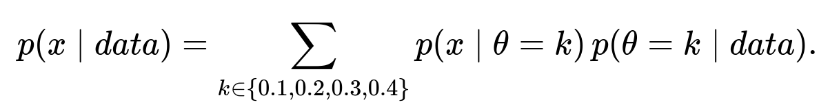
In other words, for each theta in {0.1, 0.2, 0.3, 0.4}, we compute the binomial probability of getting x sixes (because each new roll is Bernoulli with probability k), and then weight it by the posterior probability that theta = k. Summing across all k gives the posterior predictive distribution.
A subtlety arises if we only have a tiny dataset, because our posterior might still be too uncertain to give a good predictive estimate. In that scenario, the posterior probabilities might be more evenly spread among the four possible thetas. But in this problem, with 300 rolls, the posterior is strongly peaked around two values (0.2 and 0.3).
What if we suspect the data might be “contaminated” or not all 300 rolls are from the same loaded die?
In a real-world setting, there is sometimes a chance that the data does not all come from a single, consistent source. For example, perhaps someone changed the die after a certain number of rolls, or some recordings of sixes were erroneous. This scenario means the assumption “all 300 rolls share the same probability theta” might be violated.
If contamination or heterogeneity is suspected, we might need a mixture model or a more flexible hierarchical prior. Instead of a single theta for all trials, we could model a probability distribution over possible changes or drifts in theta. Alternatively, we could exclude suspected outliers from the dataset if we have reason to believe they do not reflect the same generating process.
A potential pitfall is ignoring such contamination entirely; doing so might produce artificially precise posterior estimates if the data actually arises from multiple distributions. For serious quality control or auditing, we would investigate the source of the contamination and apply robust methods that can detect or handle those anomalies.
How do we handle the situation if we do not trust the discrete set {0.1, 0.2, 0.3, 0.4} and want to add more possible values for theta?
If we believe that theta could take on more values than just the four points, we can refine our model. Instead of having exactly four discrete points, we might allow a larger finite set, say {0.05, 0.06, …, 0.45}, or even model theta as a continuous random variable (for instance, with a Beta prior). Each of these approaches broadens the model space to capture a broader range of potential probabilities for rolling a six.
When we add more possible values in a discrete prior, each value generally gets a smaller prior probability (if we keep the overall prior uniform). This can spread out the posterior as well, unless the data strongly indicates that certain values are far more likely. A pitfall here is that increasing the size of the discrete set means we may also need more computational effort to evaluate the likelihood for each possible value and normalize the posterior. However, for moderate sizes, it is still quite feasible.
How does the posterior distribution change if the observed frequency matches exactly one of the discrete theta values?
If the empirical proportion of sixes is precisely equal to one of the available theta values (for instance, if we observed exactly 30 sixes out of 100 rolls and we had {0.3, 0.35, 0.4} as possible theta values), then that particular theta will generally dominate the posterior, provided the prior is not severely biased toward other values.
In our current example (75 out of 300 is 0.25), none of the discrete points is exactly 0.25, but 0.2 and 0.3 are relatively close. If we had included 0.25 in the discrete set, it would probably become the overwhelming choice in the posterior, dwarfing 0.2 and 0.3 unless the prior was significantly larger for one of those.
What if the actual data was heavily imbalanced, for example 1 six out of 300 or 299 sixes out of 300?
In extreme scenarios, the likelihood for theta values near 0 or near 1 can dominate. For instance, if we observed only 1 six, then the empirical frequency is 1/300, which is approximately 0.0033. Even though 0.1 is still quite a bit larger than 0.0033, it is the smallest among the four discrete points in {0.1, 0.2, 0.3, 0.4}, so we would expect 0.1 to get a relatively large posterior compared to 0.2, 0.3, and 0.4. But we might also suspect none of those four values is really appropriate because they are all substantially bigger than 0.0033.
If we had 299 sixes out of 300, we would see that 0.4 is still well below the empirical proportion of 0.9967, so it might still be a poor match. This shows the importance of having a model that includes parameter values close to 0 or 1 if we think such extreme outcomes are plausible.
Can we use a loss function or a decision-theoretic approach to pick the “best” theta?
In Bayesian decision theory, after we have our posterior distribution, we can choose a point estimate for theta to minimize an expected loss. For instance, a common choice is the posterior mean if the loss is squared error. But in this discrete setting, we might choose whichever theta has the highest posterior probability if we want a mode-based decision. That is essentially the MAP (maximum a posteriori) estimate.
An alternative is to pick a risk function that penalizes being far from the true probability and compute which discrete theta minimizes that expected penalty. If the cost of being “off” by a certain margin is large, we might pick a value that is closer to the expected value of theta or some robust measure of central tendency.
What potential numerical issues can arise when computing theta^75 (1 - theta)^225 for very small or large theta?
Raising small numbers (like 0.1) to large exponents can underflow floating-point calculations in many programming languages, leading to zeros or numerical instability. Conversely, raising larger numbers to large exponents can generate overflow in extreme cases. Python’s float can handle some range of exponents, but in more constrained environments, care must be taken by working in log-space.
We often compute the log-likelihood as 75 * log(theta) + 225 * log(1 - theta) and use exponentiation only when needed to normalize. This log-sum-exp approach is a standard technique to avoid underflow/overflow. Neglecting this can lead to erroneous posterior calculations if some probabilities appear to become exactly 0 or inf in floating-point representation.
How would we handle a scenario where the prior probabilities were not all equal, say p_0(0.1) = 0.1, p_0(0.2) = 0.2, p_0(0.3) = 0.3, p_0(0.4) = 0.4?
We would simply multiply each binomial likelihood term by its corresponding prior probability (rather than 0.25 each time). For instance, the unnormalized posterior for theta=0.1 would be 0.1 * 0.1^75 * 0.9^225. Then we do the same for 0.2, 0.3, and 0.4 with their respective priors. Finally, we normalize by summing up those values and dividing.
In practice, a pitfall is to forget to renormalize after using an uneven prior. Another subtlety is that an extreme prior might overshadow the data if the sample size is small. However, with 300 rolls, the likelihood typically exerts a strong pull unless the prior is extremely skewed.
Is it possible to combine multiple experiments, each with different numbers of rolls and sixes observed, into this framework?
Yes. Bayesian updating is cumulative. If we perform a second experiment with possibly a different number of rolls and see a different count of sixes, we can update the posterior from the first experiment into a new posterior that incorporates both datasets. The key step is to multiply the old posterior (viewed as the current prior for the second experiment) by the new likelihood from the second set of data.
Concretely, if the posterior after the first 300-roll experiment is p(theta=0.1|first data), p(theta=0.2|first data), etc., we then consider the likelihood for the new data. For a second experiment with n’ rolls and x’ sixes, the likelihood for theta=0.1 is 0.1^x’ * (1-0.1)^(n’-x’), etc. Multiply these likelihoods by the old posterior probabilities and normalize to get the posterior after both experiments.
A potential pitfall is ignoring the possibility of changes in the dice or experimental conditions between the two experiments. If conditions remain the same (the same loaded die, same procedure), then it is valid to pool the data. If something changed, we would need a more complex model that allows for time-varying or condition-varying theta.