ML Interview Q Series: Estimating Exponential Distribution Rate Parameter using Maximum Likelihood

📚 Browse the full ML Interview series here.

Maximum Likelihood Estimation (Derivation): You have a set of independent observations drawn from an exponential distribution with unknown rate parameter λ. How would you derive the maximum likelihood estimator (MLE) for λ? Show the formulation of the likelihood function and the steps to obtain the MLE.

Deriving the maximum likelihood estimator (MLE) for the rate parameter λ of an exponential distribution is a foundational topic in statistics and machine learning. An exponential distribution with parameter λ (sometimes referred to as the rate parameter) has the probability density function (PDF):

Below is a detailed explanation of how to derive the MLE, with step-by-step reasoning of the formulation of the likelihood function, the log-likelihood, taking derivatives, and solving for λ. This step-by-step approach helps ensure we understand every aspect of the derivation thoroughly.

ML ESTIMATION OF λ

Likelihood Function

Log-Likelihood Function

To make calculations and differentiation more convenient, we work with the log-likelihood function ℓ(λ)=ln⁡L(λ). This transformation is strictly increasing, so maximizing the log-likelihood yields the same solution as maximizing the likelihood:

Taking the Derivative and Setting It to Zero

To find the maximum with respect to λ, we take the derivative of ℓ(λ) with respect to λ and set it equal to zero:

Setting this derivative to zero:

Solving for λ

Rearranging the above equation, we get:

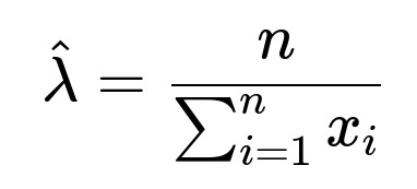
Therefore,

Second Derivative Check

For completeness, we check that this critical point corresponds to a maximum. The second derivative of the log-likelihood with respect to λ is:

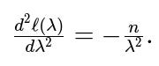
For λ>0, this is negative, indicating that ℓ(λ) is concave and the critical point we found is indeed a maximum. Thus,

is the MLE for λ under the exponential distribution.

PRACTICAL EXAMPLE WITH PYTHON CODE

Below is a quick illustration in Python on how one might compute the MLE for λ given a dataset. This snippet shows both a direct analytical solution and an example using a likelihood-based approach (though typically you would just apply the closed-form solution in practice).

import numpy as np
from scipy.optimize import minimize

# Suppose we have data drawn from an exponential with unknown rate
data = np.array([0.2, 0.5, 1.3, 0.7, 0.9, 1.1, 0.4])

# Analytical MLE solution
lambda_mle_analytical = len(data) / np.sum(data)

# Numerical approach to confirm
def negative_log_likelihood(lmbda, observations):
    # lmbda must be positive
    if lmbda[0] <= 0:
        return np.inf
    return - ( len(observations) * np.log(lmbda[0])
               - lmbda[0] * np.sum(observations) )

initial_guess = [1.0]  # some initial guess for lambda
result = minimize(negative_log_likelihood, initial_guess,
                  args=(data,), method='L-BFGS-B', bounds=[(1e-6, None)])
lambda_mle_numerical = result.x[0]

print("Analytical MLE for lambda:", lambda_mle_analytical)
print("Numerical MLE for lambda:", lambda_mle_numerical)

In almost all cases, using the closed-form solution is both exact and more efficient. However, if the model were more complicated or lacked a closed-form solution, a numerical optimization approach would be necessary.

COMMON INSIGHTS

When dealing with the exponential distribution’s parameter estimation:

Below are some follow-up questions and their thorough answers, exploring potential pitfalls and deeper concepts.

What if some of the observed data values are zero?

How would this derivation change if the exponential distribution was parameterized by its mean (θ = 1 / λ) instead?

Instead of using the rate parameter λ, one can parameterize the exponential distribution in terms of its mean θ = 1 / λ. In that case, the PDF becomes:

How does the MLE compare with the method of moments for an exponential distribution?

For an exponential distribution with parameter λ, the first moment (mean) is 1/λ. The method-of-moments estimator sets the sample mean equal to the theoretical mean:

which is exactly the same expression we got for the MLE. Thus, for the exponential distribution, the MLE and the method-of-moments estimator coincide. That is not always the case for other distributions, but for the exponential distribution, they match perfectly because the first moment directly gives us the parameter in a simple reciprocal relationship.

What are typical boundary or edge cases to consider?

3. Missing Data: If some observations are missing, one might need an EM algorithm or some imputation strategy. But under the standard complete-data scenario, the MLE formula remains straightforward.

4. Censored Data: If data is censored (e.g., you only know some observations exceed a certain threshold but not their actual values), the likelihood changes accordingly. Then you no longer have the simple closed-form MLE. Instead, you might derive a partial-likelihood function and potentially solve numerically.

Could you compare MLE and MAP (Maximum A Posteriori) estimation for λ?

While MLE uses only the likelihood of the observed data to find the parameter estimate, MAP incorporates a prior belief p(λ) into the estimation. For the exponential distribution:

How do we handle MLE for exponential distributions with incomplete or partially missing data?

If data is partially missing in a standard sense (e.g., some observations are known to be at least X but the exact values are not observed), you face a censored data problem. The solution involves:

• For each partially observed or censored sample, incorporate the probability that the sample falls in the known range. For example, if you only know a data point X is > 3, then the contribution to the likelihood is exp⁡(−λ⋅3) (the survival function at 3).

• The resulting likelihood is then a product of a PDF term for fully observed data points and a survival function term for censored data points.

• Typically, this combined likelihood no longer yields a simple closed-form MLE, so numeric methods or the EM algorithm can be applied.

Hence, the main conceptual shift is in how the likelihood is formulated for partial information, but the principle of maximizing the log-likelihood remains the same.

How would you implement a quick check for correctness of your MLE code?

One typical approach is simulation:

In Python:

import numpy as np

np.random.seed(42)
true_lambda = 2.0
n_samples = 10000

# Generate data
data = np.random.exponential(scale=1/true_lambda, size=n_samples)

# Estimate
lambda_est = n_samples / data.sum()

print("True lambda:", true_lambda)
print("Estimated lambda:", lambda_est)

For large n, you would expect lambda_est to be close to 2.0.

How can we extend this to other distributions, for instance the Gamma distribution?

For a Gamma distribution with shape k and rate θ (or scale β=1/θ), there is generally no single closed-form solution for both parameters if both are unknown. Typically, you:

This underscores why the exponential distribution (a Gamma with shape = 1) is simpler, as it has that neat closed-form solution for the MLE.

Are there any constraints on λ beyond λ > 0?

Yes, the exponential distribution requires λ > 0. Aside from that, there is no upper limit: λ can be arbitrarily large, corresponding to extremely rapid decay in the distribution. If a negative or zero value for λ appears as a potential solution, it is invalid. In both theoretical derivation and practical code, one must ensure the parameter search domain is restricted to λ > 0.

How might regularization be applied if we want to avoid extreme values of λ in the MLE estimate?

You could impose a prior on λ (e.g., Gamma prior) and perform MAP estimation. Alternatively, from a frequentist perspective, you might add a penalty term to the log-likelihood:

Final Thoughts on Estimating λ

• The derivation is straightforward: write the likelihood, take the log, differentiate with respect to λ, and solve.

• This estimator also matches the method-of-moments estimator for the exponential distribution.

• Checking for boundary cases and distribution fit is essential for real-world practice.

Once you have completed the derivation and verified that your formula or code is correct, you generally have a reliable estimate of the rate parameter under the exponential model.

---

Below are additional follow-up questions

What if the sample size is extremely small, such as n=1 or n=2?

An extremely small sample size can pose challenges when applying MLE for the exponential distribution. In theory, the MLE formula

remains valid even for small n. However, there are some subtle practical and conceptual issues:

• n=1: If you have a single observation ( x_1 ), the MLE becomes

• This is still valid but can be heavily influenced by outliers in either ( x_1 ) or ( x_2 ). One small measurement drastically raises ( \hat{\lambda} ).

• Interpretation and Variance: The MLE for (\lambda) with very small n has high uncertainty. A single or couple of data points do not robustly represent the underlying distribution. In practice, you might:

  • Use Bayesian methods with a reasonable prior to stabilize estimates.

  • Collect more data if possible.

  • Provide confidence intervals or credible intervals, which often show that the uncertainty is large.

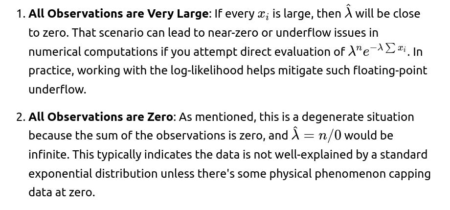
• Edge Case: If either observation is 0 (in the n=2 scenario) or your single observation is 0 (in the n=1 scenario), the sum of observations can be 0, pushing ( \hat{\lambda} ) to infinity in a purely theoretical sense. This highlights how fragile the estimate can be for tiny samples.

Hence, while mathematically valid, the MLE with extremely small n can be very unreliable. Additional data or prior knowledge is strongly recommended.

How does the MLE behave if the data is not truly exponential but we force an exponential assumption?

When the true underlying distribution is not exponential, forcing an exponential model can lead to systematic bias or poor predictive performance. Potential scenarios include:

• Heavier-Tailed Data: If the true data is from a distribution with a heavier tail (e.g., a Pareto or some heavy-tailed mixture), the MLE for (\lambda) could underestimate the tail probability, because an exponential distribution decays faster than heavier-tailed distributions. Long, infrequent observations stretch the sum ( \sum x_i ), causing a smaller (\hat{\lambda}).

• Lighter-Tailed Data: If the true data distribution is short-tailed (e.g., bounded or sub-exponential), the exponential assumption may overestimate the frequency of large values. You might see a larger (\hat{\lambda}) than is consistent with the actual phenomenon.

• Mixture of Exponentials: Real processes can combine different rates. For instance, you might have a mixture of shorter waiting times and longer waiting times. A single-rate exponential might not fit well, and the MLE tries to find a compromise rate parameter that often doesn’t capture the multi-modal nature of the data.

• Model Diagnostics: In real applications, you should assess goodness-of-fit. For example:

  • Kolmogorov-Smirnov Test for exponential distribution.

  • QQ-plots or PP-plots to visually check how well your data aligns with the exponential model.

  • Likelihood ratio tests if you compare exponentials with more flexible distributions (e.g., Gamma).

Ultimately, if the data is not exponential, the MLE is simply maximizing the likelihood under the wrong model. It still yields a mathematical best-fit under that assumption, but the results and subsequent inferences could be misleading.

How do outliers or extreme values affect the exponential MLE?

In an exponential distribution, large observations (outliers) can significantly affect the sum of all observations and thereby reduce (\hat{\lambda}). Some real-world implications:

• Long-Tail Sensitivity: Since (\hat{\lambda} = n / \sum x_i), even a single large ( x_i ) can increase ( \sum x_i ) substantially, leading to a smaller estimate of (\hat{\lambda}). This might create an unrealistic expectation that large observations are relatively common or that the average rate is slower.

• Robustness Concerns: The exponential MLE is not particularly robust to outliers because it weighs every data point equally in the sum. If outliers are truly part of the data-generating process, that’s appropriate. If outliers result from data entry errors or anomalies outside the normal scope, the MLE may become skewed.

• Practical Handling:

  • Data Cleaning: Verify that outliers are valid. If some are errors, correct or remove them.

  • Alternative Distributions: If outliers are valid but frequent, consider heavier-tailed distributions (e.g., Pareto, Lognormal, Gamma with shape parameter < 1).

  • Robust Estimation: Alternatively, use robust procedures or incorporate prior knowledge (Bayesian) that moderates the effect of extreme values.

Thus, while the exponential MLE works well for data that genuinely follows an exponential distribution, outliers can heavily distort the parameter estimate if the data do not conform to that assumption.

How do we construct a confidence interval for the MLE of λ?

A common technique to derive a confidence interval for the exponential rate (\lambda) uses either the asymptotic normality of the MLE or direct transformations:

1. Asymptotic Normality: For large n, the MLE (\hat{\lambda}) is approximately normally distributed around the true (\lambda), with a variance given by the inverse of the Fisher information. For the exponential distribution, the Fisher information for (\lambda) with n samples is

Hence, the variance of (\hat{\lambda}) is

Substituting (\hat{\lambda}) for (\lambda):

A rough (1-(\alpha)) confidence interval can be written as

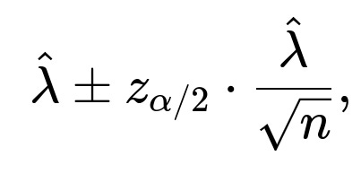
where (z_{\alpha/2}) is the standard normal critical value.

2. Likelihood Ratio Methods: Another approach is to use the profile likelihood for (\lambda) and find the interval where the log-likelihood stays within a certain cutoff from its maximum. This method can be more accurate for smaller n.

3. Exact or Pivot-Based Intervals: For exponential data, it’s also possible to use the fact that (\sum x_i \sim \text{Gamma}(n, \lambda)). Then you can construct an exact confidence interval for (\lambda) leveraging Gamma distribution quantiles:

   • If ( T = \lambda \sum_{i=1}^n x_i \sim \chi^2_{2n} ) (because a Gamma with shape n can be related to a (\chi^2) distribution), you can invert that relationship to find confidence limits that do not rely on large-sample approximations.

Practical Usage: In typical large-sample scenarios, the asymptotic approach is straightforward and works well. For smaller samples, the exact or likelihood-ratio-based intervals are more accurate but require more computation (e.g., numerical root-finding or table lookups).

How do we handle scenarios where λ might change over time?

In many real-world processes, the rate parameter (\lambda) is not constant. For instance, the time between events may shorten or lengthen over different phases. An exponential distribution with a single (\lambda) becomes a poor fit if the process is non-stationary. Some strategies:

• Piecewise Exponential Model: Split the observation timeline into segments where (\lambda) is assumed constant within each segment but can differ across segments. Then you estimate separate MLEs (\hat{\lambda}_1, \hat{\lambda}_2, \dots) for each segment.

• Non-Homogeneous Poisson Processes (NHPP): In continuous-time event processes, you can model a rate function (\lambda(t)) that varies with time. The likelihood involves integrating (\lambda(t)) over each event's time interval. You often must resort to numeric methods or specialized assumptions (e.g., a piecewise constant (\lambda(t)) or a parametric form like (\lambda(t) = \alpha + \beta t)).

• State-Space Models: If (\lambda) changes stochastically, you can use Bayesian or state-space approaches that treat (\lambda) as a latent variable evolving over time (e.g., a random walk or a dynamic linear model).

• Practical Note: If you simply lump all data and assume a single (\lambda), you might get an average rate that fails to capture the true temporal variations, leading to poor predictions or misinterpretation of event dynamics.

Could we use the exponential MLE as a stepping stone in a hierarchical or multi-level model?

Yes. In certain hierarchical setups—say you have multiple groups or conditions each believed to follow an exponential distribution but sharing some global hyperparameters—you might do the following:

• Estimate (\lambda) for each group independently using MLE or a Bayesian approach.

• Then place a higher-level prior on (\lambda) across groups if the group rates are somewhat related. For example:

  • Hyperprior: You might assume (\lambda) for each group is drawn from a Gamma distribution, forming a Gamma-Gamma hierarchical model (since an exponential is a Gamma with shape=1).

  • Partial Pooling: If each group has limited data, pooling across groups can help stabilize the parameter estimates. You might find that group-specific (\lambda_i) shrinks toward a global mean.

Though the direct MLE from each group is not always the final solution in hierarchical modeling, it can serve as an initial guess or an input to an iterative method (like an EM algorithm or Hamiltonian Monte Carlo in a Bayesian setting). The key is that MLE for the exponential rate in each subgroup is easy to compute, providing a quick baseline or starting point for more complex multi-level models.

What if the data has been discretized or rounded, but we still assume an exponential model?

Real datasets often measure time in discrete units (e.g., hours, days) rather than exact continuous values. Technically, the exponential distribution is a continuous model, so how do we handle discretization?

• Direct Mismatch: If the data is purely discrete, using a continuous PDF can introduce bias. The MLE formula

might still be used as an approximation if the discretization is fine (e.g., measuring times in milliseconds for events that typically last seconds).

• Interval Censoring: Rounding can be seen as a form of interval censoring (each true value is in an interval [k, k+1) if rounding to the nearest integer). The correct approach is to write down the probability that a time belongs to that interval under the exponential model and maximize the corresponding likelihood. That typically necessitates a more involved likelihood function:

  • The probability of rounding to integer k is

for each observed integer k.

• You then multiply these probabilities for all data points and solve numerically for (\lambda).

• Practical Approach: If the rounding is minor or the time scale is small compared to typical event durations, many practitioners still apply the continuous MLE as an approximation. If the rounding is coarse (e.g., rounding to days, but typical durations are hours or minutes), the mismatch can become significant, and a discrete-likelihood approach is preferred.

In short, the standard MLE formula might not be strictly correct for heavily discretized data. A more sophisticated approach or a discrete analog of the exponential distribution (like the geometric) might fit better.

How do we validate or stress-test the MLE in simulation frameworks?

A useful practice is to simulate data from known parameters and compare the estimated (\hat{\lambda}) to the true (\lambda). Several approaches include:

• Monte Carlo Replications: Repeatedly sample data sets of size n from (\text{Exponential}(\lambda_0)). For each dataset, compute the MLE (\hat{\lambda}). Track the distribution of (\hat{\lambda}) across many simulations. Evaluate:

  • Bias: On average, does (\hat{\lambda}) differ significantly from (\lambda_0)? For the exponential distribution, the MLE is unbiased for large n (and even for moderate n, the bias is usually small).

  • Variance: Check how spread out the estimates are. Compare with the Fisher information or known variance formula.

  • Coverage: If constructing confidence intervals, see whether they contain (\lambda_0) at the nominal rate (e.g., 95% coverage).

• Stress Tests: Add noise or contamination to the simulated data. For example, generate 90% from an exponential with (\lambda_0) and 10% from a different distribution. Examine how sensitive (\hat{\lambda}) is to that contamination.

• Implementation Verification: This is an excellent way to confirm that your coding approach (if you are doing numeric maximization or partial likelihood for censored data) matches the known theoretical solution.

Simulation is often the gold standard for verifying theoretical estimators and identifying unexpected issues before applying methods to real data.

How can we interpret the memoryless property in relation to MLE?

A hallmark of the exponential distribution is the memoryless property: the remaining waiting time distribution does not depend on how long you have already waited. Formally, for ( X \sim \text{Exponential}(\lambda) ), we have:

• ( P(X > s + t \mid X > s) = P(X > t). )

In practical terms:

1. Data Collection: If you suspect a memoryless process (e.g., time between arrivals in a Poisson process), the exponential assumption might be appropriate, and then MLE for (\lambda) is straightforward. However, if you observe that the distribution of remaining times depends on how long you have already waited, the exponential assumption is violated.

2. Interpretation of (\hat{\lambda}): The MLE rate (\hat{\lambda}) suggests that on average, the event rate is constant over time and does not “remember” how much time has already elapsed.

3. Diagnostic: A standard check is to see if the memoryless property is approximately correct. One approach is plotting or testing that

1. If that ratio clearly varies with s, the memoryless assumption is not holding, indicating a poor exponential fit.

Thus, if data is truly memoryless, the MLE for (\lambda) should be not only mathematically convenient but also conceptually correct. If memoryless behavior is not observed, even the correct MLE might be modeling the data incorrectly.

How might boundary constraints or domain knowledge about λ be incorporated into the MLE?

Although the exponential MLE does not require additional constraints beyond (\lambda > 0), in some applications you might have domain knowledge indicating that (\lambda) cannot exceed a certain maximum or must be above some minimum. For instance:

• Physical Constraints: In certain reliability contexts, you may know events cannot occur more often than once per second, placing an upper bound on (\lambda).

• Economics or Queuing: If you know your arrival rate (\lambda) is within a specific range, you could limit your parameter search to that interval.

To incorporate such constraints:

• Constrained MLE: Solve the log-likelihood maximization subject to ( \lambda_{\min} \le \lambda \le \lambda_{\max} ). If the unconstrained MLE falls within that interval, no change is necessary; otherwise, you choose the boundary. For exponential distributions, the unconstrained MLE is ( n / \sum x_i ). If that value is below (\lambda_{\min}), the constrained MLE is (\lambda_{\min}). If it is above (\lambda_{\max}), the constrained MLE is (\lambda_{\max}).

• Penalty Methods: Alternatively, you could use a soft penalty in the objective function that heavily penalizes (\lambda) outside the domain. That is effectively a “soft” way to keep (\lambda) near an acceptable range.

• Bayesian Prior: Domain constraints can also be expressed as a prior distribution. For instance, a truncated Gamma prior that disallows values outside a certain range. Then MAP estimation or posterior sampling would incorporate that information automatically.

Such constraints might be crucial in real-world engineering systems or economic models where certain rates are physically impossible. Simply applying the unconstrained MLE might yield an implausible estimate otherwise.