
ML Interview Q Series: Estimating Pi Using the Monte Carlo Simulation Method
Browse all the Probability Interview Questions here.
21. Estimate π using a Monte Carlo method. (Hint: think about throwing darts on a square and seeing which land inside the circle.)
Here is a detailed explanation of how to estimate π using a Monte Carlo simulation, along with thorough discussions of the reasoning and the important considerations you might encounter in a FANG-level interview. The essential idea behind this method is to simulate random “dart throws” into a square that encloses a circle, then measure the ratio of darts that land inside the circle to total darts thrown. This ratio, multiplied appropriately, provides an estimate of π.
Core Concept and Mathematical Relationship
We consider a circle of radius 1 centered at the origin. This circle will be entirely contained within a square of side length 2 (with corners at (-1, -1), (-1, 1), (1, 1), and (1, -1)).
If we randomly and uniformly sample points within that square, the probability that a point lies inside the unit circle is the ratio of the area of the circle to the area of the square. The area of the circle with radius 1 is π, while the area of the square is 4. Therefore, the probability of landing inside the circle is π/4. If we denote by N_total the total number of random points (darts) and by N_inside the number of points that fall inside the unit circle, we can approximate π via:

In practice, we generate a large number of (x, y) points uniformly in the square [-1, 1] × [-1, 1], check whether x² + y² ≤ 1 (which implies the point is within the circle), count how many such points satisfy this condition, and compute π based on the above ratio.
Practical Implementation in Python
Below is a Python code snippet illustrating how to estimate π using this Monte Carlo approach. We use random points in the square [-1, 1] × [-1, 1]. Each point that satisfies x² + y² ≤ 1 lies inside the circle. The ratio of these inside points to total points, multiplied by 4, approximates π.
import random

def estimate_pi(num_samples):
    inside = 0
    for _ in range(num_samples):
        x = random.uniform(-1, 1)
        y = random.uniform(-1, 1)
        if x**2 + y**2 <= 1:
            inside += 1
    pi_estimate = 4 * inside / num_samples
    return pi_estimate

# Example usage:
samples = 1_000_000
pi_approx = estimate_pi(samples)
print(f"Estimated π after {samples} samples: {pi_approx}")
This code illustrates the basic Monte Carlo routine. The more samples you use, the closer you typically get to the true value of π, although the exact difference to the true π value shrinks statistically with the square root of the number of samples (due to the Law of Large Numbers and the Central Limit Theorem).
Explanation of Key Steps
Throwing Darts Uniformly
To ensure the Monte Carlo estimate converges properly, we must draw samples (x, y) uniformly from the square. In the above code, random.uniform(-1, 1) draws a floating-point number uniformly in the interval [-1, 1]. If the distribution is not truly uniform, or if there is any bias in the random sampling, the π estimate will reflect that bias.
Inside-Circle Check
We check if the dart lies inside the unit circle by computing x² + y². For a point to be inside the circle (radius = 1), we need x² + y² ≤ 1.
Ratio of Areas
The logic that π = (Area of Circle) / (Area of Square) × 4 is at the heart of why the ratio of points inside the circle versus total points corresponds to π/4.
Discussion of Convergence and Accuracy
As the number of samples increases, the Monte Carlo estimation of π will converge to the true value of π (in a statistical sense). Specifically, the standard error of a Monte Carlo estimate typically shrinks proportionally to 1/√(N_total). In practical terms, this means we need on the order of millions of samples to see the estimate reliably settle in near 3.14–3.15.
Monte Carlo methods are thus often slower to converge than other deterministic approximation techniques (for instance, certain infinite series expansions), but they are easy to implement, conceptually straightforward, and apply to many other problems well beyond just approximating π.
Addressing Potential Follow-up Questions
Below are several follow-up questions that an interviewer might ask to test deeper knowledge about this method, random sampling, and more sophisticated issues that can arise in real-world machine learning or scientific computing. Each follow-up question is shown in H3 format, followed by an in-depth answer.
How does the random seed or generator quality affect the Monte Carlo estimate?
If the random number generator (RNG) is poor or exhibits patterns, the samples might not be uniformly distributed, and you could get a skewed estimate of π. In practice, you should use a well-tested RNG (for instance, Python’s built-in Mersenne Twister is generally acceptable for basic Monte Carlo simulations, but for cryptographic or highly sensitive simulations, more robust RNGs might be used). It is also common to set a seed for reproducibility, but the randomness quality still matters for accuracy and convergence.
How many samples do we typically need for a given level of accuracy?
A standard rule-of-thumb for Monte Carlo approaches is that the error decreases on the order of 1/√N. If you need an absolute error of about 0.001 (for π ≈ 3.1415926535...), you might perform the following rough estimate:
Let the standard deviation of the Bernoulli process (inside vs. outside the circle) be σ. For a circle within a square, one can roughly approximate σ to be on the order of √(p(1 − p)), where p ≈ π/4. Then the standard error on the fraction p is roughly √(p(1 − p)/N). When you multiply this fraction by 4 to get π, the error scales similarly with 1/√N. So you’d need at least in the hundreds of thousands or millions of samples to reliably see the 0.001 level of accuracy.
Could we use a different geometric shape or approach?
Yes. You could choose a quarter of a circle, or an eighth, or any shape whose area we know relative to the entire region from which we sample. In most practical implementations, it is simply easiest to use the full circle in the square. However, some might prefer sampling just the first quadrant [0, 1] × [0, 1] and looking at the quarter of the circle. Both approaches are mathematically valid, but using just the first quadrant might reduce the range of the uniform calls a bit. Ultimately, the difference is minimal for large N, though subtle numerical performance differences can occur in certain languages or libraries.
Are there more efficient or deterministic methods to approximate π?
Yes. Infinite series expansions (like the Gregory–Leibniz series) or other numerical integration methods can yield faster convergence. For instance, the Gregory–Leibniz series:
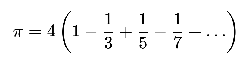
converges, but rather slowly. Other series converge much more quickly (e.g., the Machin-like formulas). The Monte Carlo method, while straightforward, is not the most efficient for approximating π alone. However, its significance is that Monte Carlo generalizes readily to high-dimensional integrals, where it often becomes more practical than deterministic methods.
What are some common pitfalls or implementation errors?
A common pitfall is using a poor RNG or forgetting to initialize the random seed, which can lead to unintentional biases or lack of reproducibility. Another pitfall is sampling from the wrong domain or miscounting the points that lie inside the circle. Also, confusion can arise if someone calculates the boundary incorrectly, for example checking x² + y² < 1 instead of x² + y² ≤ 1 is typically not a big difference, but it can cause minor discrepancies in very large-scale runs.
How can we parallelize or speed up this simulation?
Because each dart throw is independent, we can parallelize the simulation easily by splitting the total number of samples into batches. For instance, we could run multiple threads or processes, each of which computes how many points land inside the circle out of some subset of samples, and then aggregate the results. In Python, we might use multiprocessing or libraries such as Dask or Ray for large-scale computations. This parallelization is straightforward and one of the strengths of Monte Carlo methods.
What if we wanted to adapt this method to higher dimensions?
In higher dimensions, we would approximate the volume of an n-dimensional hypersphere by sampling points in an n-dimensional hypercube. The fraction of points lying inside the hypersphere gives the ratio of their volumes. The same principle still applies, but the shape is an n-dimensional sphere, and the volume is

. As the dimension grows, the fraction of points that land inside the hypersphere diminishes quickly, so the problem can become more challenging in practice, and variance can grow. This phenomenon is one example of the “curse of dimensionality.” Nonetheless, Monte Carlo is one of the few methods that can still handle such high-dimensional integrals, although it may converge more slowly without variance-reduction techniques.
Can this approach yield insights into randomness and distribution properties?
Yes. Beyond simply estimating π, analyzing how fast or slow the estimate converges, or how it fluctuates, can provide insights into the distribution of your random samples. You can inspect if the distribution is uniform or if there is any clustering (e.g., potential issues with pseudorandom generators). Plotting the points can reveal patterns or irregularities that might need further investigation.
How can variance reduction help?
Variance reduction techniques like importance sampling, stratified sampling, or antithetic sampling can be used to reduce the variance of Monte Carlo estimates in more complex integrals. For a simple circle-in-square experiment, these techniques may not provide a dramatic benefit, but they illustrate the principle that Monte Carlo can be enhanced with smarter sampling approaches. For instance, stratifying the square into subregions and forcing the simulation to sample a fixed number of points in each subregion can help ensure consistent coverage, which might lead to slightly less variance in practice.
What if we tested partial ranges instead of the entire circle all at once?
One could, for instance, split the domain into symmetrical regions (like four quadrants or eight wedges) and estimate partial areas. You would then sum these partial areas or partial probabilities to get an overall estimate of π. This modular approach can sometimes help with parallelization or with diagnosing numerical issues, especially if one region is systematically being under-sampled.
How does the Law of Large Numbers and Central Limit Theorem apply here?
The Law of Large Numbers ensures that, as the number of samples grows large, the empirical ratio of points inside the circle converges to the true probability (π/4). The Central Limit Theorem tells us that the distribution of the average (or sum) of i.i.d. random variables—such as Bernoulli indicators for whether a point is inside or outside the circle—approaches a normal distribution for large sample sizes. This is why the error bars on the Monte Carlo estimate have a roughly 1/√N behavior.
Could this approach be used in a real production system?
In practice, one rarely builds a production system solely to estimate π this way, since π is known to many decimal places. However, Monte Carlo is extensively used in production for risk management, probabilistic modeling, simulations in finance and physics, and so on. The π example is simply a canonical illustration of the method. Should you use Monte Carlo for something else in production, you would take care to manage the random seed for reproducibility, potentially apply variance reduction, and consider multi-threading or distributed computing for large-scale tasks.
Conclusion
The Monte Carlo approach to estimating π is an elegant demonstration of random sampling techniques. It showcases the fundamentals of probabilistic estimation, convergence rates, and the role of random number generators. By understanding these basics—throwing darts uniformly, checking if they’re within the circle, and scaling the ratio by 4—you get a straightforward estimation of π. Though not the fastest method to compute π, it remains one of the best-known and most conceptually simple examples of Monte Carlo simulation methods.
In a FANG-level interview, expect deeper discussion on randomness, convergence, error analysis, and possible pitfalls in large-scale or high-dimensional scenarios. Demonstrating you understand these subtleties shows an interviewer that you not only know the basic algorithm, but also the advanced concepts and real-world considerations behind Monte Carlo methods.
Below are additional follow-up questions
What happens if we place the circle off-center within the square instead of centering it at the origin?
If the circle’s center is no longer at (0, 0) but somewhere else, the fundamental idea remains the same: we sample points within a known bounding region that encloses the circle and check how many samples lie inside it. However, we must be certain that our bounding region is strictly larger than or equal to the circle in question. Instead of using x² + y² ≤ 1 to check if a point lies in the circle, the check would become (x - x_center)² + (y - y_center)² ≤ r² if the circle has radius r and center at (x_center, y_center).
The key difference is that if the circle is no longer at the origin, we have to adjust our random-sampling domain to ensure it properly covers the circle (e.g., if the circle is partially outside the original square). If the circle is still fully within [-1, 1] × [-1, 1] but simply shifted, the bounding box might remain the same size (2 × 2), but we must update the sampling formula for x and y so that the random points match the correct domain.
One subtle point is to verify that you know exactly how large the bounding square should be if the circle’s shift causes it to protrude beyond the original square. If you accidentally sample from an incorrect bounding region that doesn’t fully contain the circle, you get an underestimation or overestimation of π, depending on how that mismatch is handled.
A potential pitfall is forgetting to use the correct bounding region dimension. For example, if the circle is centered at (0.5, 0), you might erroneously still sample from [-1, 1] in both x and y, which would yield an incorrect probability if the circle extends outside the region on one side.
Another issue is increased computational overhead for checking whether a point is inside the circle if you embed it in a bounding region that is substantially larger than necessary. Sampling from an unnecessarily large region may increase variance because the ratio of circle area to bounding region area becomes smaller, making it harder to accurately estimate π with a given number of samples.
If you want to stick to the simplest approach, you can still center at (0, 0). But in scenarios where the circle’s position is meaningful for the simulation, you adapt the sampling logic accordingly, ensuring you capture the entire circle without error.
How might floating-point precision limitations affect the Monte Carlo estimate in large-scale simulations?
When estimating π with very large numbers of samples (possibly in the billions), floating-point precision can become an important consideration. In languages like Python, floating-point numbers typically follow IEEE 754 double precision, which gives a large range but is still subject to rounding errors:
If we sample a huge number of points, counters such as N_inside can grow very large. Division operations for inside / total might lose a bit of precision if not done carefully. Typically, with double precision floats, normal Monte Carlo estimates of π are not severely affected until extremely high numbers of samples. However, subtle accumulation of floating-point rounding could cause minor bias.
Another floating-point issue arises when dealing with x² + y² if x and y are extremely small or extremely large. In standard Monte Carlo on a [-1, 1] range, overflow or underflow is unlikely, but if for some reason the radius or domain were scaled up or if you were simulating random points with very large magnitude, you could face numeric instability. For instance, if x and y are on the order of 10^10, squaring them leads to 10^20, which might push the floating-point representation to its limits, depending on how it’s computed.
One way to mitigate floating-point issues is to track the inside count and total count as integers (which Python can handle to arbitrary size) and only perform floating-point division at the end. This ensures the ratio is calculated in a single step and is less prone to incremental rounding errors. Another strategy is to use libraries designed for extended precision arithmetic, though that is rarely necessary for standard Monte Carlo estimates of π.
Can we use quasi-random sequences instead of pseudorandom sequences, and how would that affect the estimate?
Quasi-random sequences (also called low-discrepancy sequences) such as the Sobol or Halton sequences are specifically designed to fill a space more uniformly than purely pseudorandom sequences. Instead of relying on statistical randomness, these sequences aim to systematically reduce the gaps and clusters that can occur with ordinary pseudorandom draws.
In a Monte Carlo estimate of π, switching to quasi-random sampling generally reduces the variance of the estimate for a given number of points. You might see the estimate converging to π more smoothly compared to using standard pseudorandom draws, where you can have noticeable fluctuations even for moderately large numbers of samples.
A potential pitfall with quasi-random sequences is that they are deterministic in nature. If you are relying on strict randomness for reasons other than merely computing an integral (for example, in certain randomized algorithms that need random bits for security or certain sampling-based proofs), quasi-random sequences might not be suitable. Another subtlety is that while quasi-random sequences can improve convergence in low to moderate dimensions, in very high-dimensional scenarios, the benefits might not be as pronounced without careful tuning.
In practical applications, many HPC (High Performance Computing) frameworks or advanced scientific libraries offer direct ways to generate these sequences, making it straightforward to replace pseudorandom sampling with quasi-random approaches and observe better convergence properties.
How does the acceptance-rejection method compare to the dart-throwing approach?
The dart-throwing approach to estimate π is essentially a form of acceptance-rejection sampling, where the “proposed” distribution is a uniform distribution over the square, and you accept a sample if it falls inside the circle. In a more general acceptance-rejection framework, you want to sample from a complex target distribution by first sampling from a simpler proposal distribution and deciding whether to accept the point according to a certain criterion.
In the context of estimating π, the circle is the region you want to “accept,” and the square is your proposal region. The acceptance probability is the ratio of the circle area to the bounding region area.
When comparing to more advanced acceptance-rejection scenarios, potential pitfalls include:
• Choosing a bounding region that is too large relative to the circle (or in other applications, relative to the target distribution), leading to a high rejection rate and increased variance. • Failure to ensure the proposal distribution properly covers the region of interest, causing a biased or incomplete sampling of the shape.
For estimating π specifically, the method is so direct that acceptance-rejection is effectively the same as the standard Monte Carlo approach. But in more complicated integrals or multi-dimensional shapes, acceptance-rejection can suffer from poor efficiency if there is a big difference between the volume you sample from and the volume of interest.
How can we handle a scenario where our distribution of dart throws is not uniform?
If the random “dart throws” are not uniform over the square, the straightforward formula π ≈ (4 × N_inside) / N_total may no longer hold. Monte Carlo methods for integration rely on the assumption that sampling is uniform (or at least that the sampling density is known and can be accounted for).
If you cannot guarantee uniform sampling but you know the sampling density function f(x, y), you can still estimate integrals by weighting each sample appropriately. Instead of simply counting the fraction of points in the circle, you would sum up an indicator function that the point is inside the circle, normalized by the probability density at which that point was drawn.
Concretely, the estimate of π might become an integral of the indicator function inside the circle over the sampling density. You would do something like:

where f(x_i, y_i) is the density of your sampling distribution and (\mathbf{1}(\cdot)) is the indicator function. The exact expression depends on how you normalize for the bounding region’s total probability mass. The point is that if you deviate from uniform sampling, you must incorporate knowledge of the density function in your estimator to ensure correctness and avoid bias.
A common pitfall is to ignore this and simply count the inside fraction as if the sampling were uniform. You’ll end up with an incorrect value of π, possibly off by a large margin if the distribution deviates significantly from uniform. In real-world scenarios, sometimes non-uniform sampling is used to reduce variance in more complicated integrals, but you have to do it in a principled way (importance sampling) to preserve correctness.
How could we incorporate real-time updates of the estimate if the Monte Carlo simulation is being run interactively?
In an interactive or streaming scenario, you might want to see how the estimate of π evolves in real time as samples continue to arrive. You can maintain running totals of N_inside and N_total as more points are generated. After every new dart throw, or after each batch of them, you update:
inside_count += 1 if x² + y² ≤ 1 total_count += 1
Then you compute:
ParseError: KaTeX parse error: Expected 'EOF', got '_' at position 62: …es \text{inside_̲count}}{\text{t…
As points accumulate, the estimate typically stabilizes (though it will still fluctuate due to randomness). In practice, you can also maintain a running confidence interval using approximate normality for large sample sizes. For each sample, consider the Bernoulli outcome of “inside circle or not.” Then you can apply:
• The sample mean: ( \hat{p} = \frac{\text{inside_count}}{\text{total_count}} ) • The sample variance for Bernoulli((\hat{p})) is ( \hat{p} (1 - \hat{p}) ).
Hence, a 95% confidence interval for p is roughly:
ParseError: KaTeX parse error: Expected 'EOF', got '_' at position 63: …})}{\text{total_̲count}}}
Since (\pi = 4 \times p), we just scale those bounds by 4 to get a confidence interval for π.
A subtlety is that you must trust your random draws are truly random and that the ratio of inside_count to total_count is indeed a valid Bernoulli process across draws. If the distribution or process changes over time (e.g., you are changing how you sample or the circle radius changes mid-simulation), then the streaming approach to a stable estimate might not be valid, and you’d have to restart or segment the computation carefully.
What additional considerations should we have if we run on a GPU or other hardware accelerators?
Using GPUs for the Monte Carlo simulation can accelerate the generation of random numbers and the inside-circle checks. This is straightforward if you use libraries like CUDA in C++ or frameworks in Python (such as PyTorch or CuPy) that offer GPU-accelerated random sampling.
However, when parallelizing across many GPU threads, you must ensure:
• Each thread has access to a quality random number generator that is independent from other threads. Many GPU frameworks provide well-tested parallel RNG solutions, but if you use them incorrectly (for instance, forgetting to properly set unique seed states for each thread), you might introduce correlations between threads. • The overhead of transferring final counts back to the CPU or performing inter-thread reductions can become a bottleneck if not designed well. Typically, you’d perform a parallel reduction on the GPU to sum the inside results and then copy a single aggregated value back. • The partial sums from each thread must not overflow integer limits. Usually, that is not a problem if you store results in a 32-bit or 64-bit integer, but extreme-scale runs should be mindful of this.
Potential pitfalls include subtle concurrency issues where multiple threads attempt to update the same global counter simultaneously without atomic operations. This can lead to race conditions or inaccurate counts of inside points. A more robust strategy is to give each thread its own local counter and then sum them all in a second pass.
How can we extend the approach if instead of a circle, we have an irregularly shaped target region whose area we still want to estimate?
The generalization to any shape of interest is straightforward conceptually: if the shape’s bounding box (or bounding region) is known and you can sample points uniformly inside that bounding region, the fraction of points landing in the shape times the bounding region area gives an estimate of the shape’s area. For a 2D shape, it’s area; for a 3D shape, it’s volume, and so forth.
The challenge with irregular shapes is efficiently checking membership. For a circle, we have a simple x² + y² ≤ r². For a polygon, you might use ray casting or the winding number technique to check whether a point is inside. For more complex geometries, you may need advanced computational geometry algorithms. The more computationally expensive the membership check is, the more you might want to reduce variance using better sampling approaches (for instance, adaptive sampling around the shape boundaries).
In an interview setting, you might be asked how to do this for very complicated shapes in higher dimensions. You’d note that as dimensionality grows, the volume of the bounding box can vastly exceed that of the shape, causing the fraction of “inside” points to become very small. This leads to high variance unless you use importance sampling or partition the region cleverly. That phenomenon is another illustration of the curse of dimensionality, where high-dimensional Monte Carlo computations can become inefficient without specialized techniques.
Could we incorporate a performance metric, such as time to achieve a certain desired accuracy?
Performance in Monte Carlo often focuses on how long it takes to reach a given error tolerance. For π estimation, we might define a target accuracy, say ±0.0001. One can theoretically derive how many samples are needed to reach that target with high probability based on standard error approximations from the Central Limit Theorem. Then, if you know your hardware’s sampling rate (e.g., X million samples per second on the CPU or GPU), you can estimate the runtime.
You might also implement a stopping criterion: continuously compute the estimate of π and track the running standard deviation or confidence interval. Once the interval is narrower than the target precision, you stop. This is sometimes called an “any-time algorithm” because it can provide progressively refined answers without a pre-fixed sample size.
A subtle point is that because the Monte Carlo estimate is random, even after many samples, you can still see random fluctuations outside your desired range. The stopping criterion typically relies on probabilistic bounds (e.g., we are 95% confident our estimate is within ±0.0001 of π). True guaranteed bounds would require a more conservative approach.
Another subtlety is that if your random generator or sampling method changes mid-run (e.g., a shift from CPU-based to GPU-based sampling or a change in seeds), your distribution might be disrupted, invalidating the typical assumptions behind the standard error calculations. Ensuring a consistent sampling method throughout is key for a well-defined stopping criterion.
How do we deal with correlated samples if, for instance, we use a Markov chain approach?
In some Monte Carlo methods (like Markov Chain Monte Carlo, MCMC), the samples are not independent but correlated. For the basic π estimation example, it’s unusual to use MCMC because we can sample uniformly in the square without needing a Markov chain. However, if for some reason you employed an MCMC technique (maybe because in a broader scenario you’re sampling from a complicated distribution and approximating some geometric property), the correlation between successive samples complicates the variance analysis.
The Central Limit Theorem still often applies, but you have to account for the effective sample size being lower than the raw number of draws. Correlated samples may cluster and cause slow exploration of the space, leading to slower convergence for the area or volume estimate.
One subtle issue is ensuring that your Markov chain actually has a stationary distribution matching the domain of interest (e.g., uniform over the square). If your chain has not reached stationarity, early samples may bias the estimate. In practice, one uses “burn-in” steps to allow the chain to approach its stationary distribution and discards those early samples. If you don’t handle burn-in properly, your estimated value of π might be systematically biased.
Another subtlety is that you can reduce correlation by thinning (picking every nth sample) or by using multiple independent chains. While these techniques can reduce correlation, they might also throw away potentially useful data or require extra computational cost.
What special considerations arise if the random draws are from a physical (hardware) random generator?
Some systems use hardware random number generators (HRNG), perhaps based on thermal noise or quantum phenomena, rather than purely algorithmic pseudorandom generators. The advantage is that the randomness is theoretically “true” and not just a deterministic sequence. For most Monte Carlo simulations (including π estimation), pseudorandom is sufficient. However, in certain cryptographic contexts or high-stakes simulations, physical randomness might be preferred.
Potential pitfalls include verifying that the hardware generator is unbiased and stable. If the hardware fails or drifts over time, the distribution may shift away from uniform. This could go unnoticed, introducing error into the π estimate. In an interview, you might mention that controlling for and calibrating hardware RNG outputs is more challenging than using a well-studied pseudorandom algorithm, which is typically stable and reproducible.
You could do randomness tests (e.g., NIST randomness tests) on your hardware-based sequence to detect anomalies. Even then, hardware sources can degrade or be tampered with, introducing subtle biases. For a simple simulation like π, these biases might be small, but in a setting where absolute correctness is crucial, thorough verification is recommended.
How does discretization or “grid” sampling differ from random sampling for estimating π?
Sometimes, instead of drawing random points, people might attempt to lay down a fine grid and count how many grid points fall inside the circle. This is more akin to a Riemann sum or a deterministic integration approach. It can converge to the true area, but the rate of convergence depends on how fine the grid is. Each grid point typically represents a small cell in the square, and we can approximate π by the fraction of cells that lie inside the circle times the total area.
A potential advantage of the grid approach is that it has no randomness and might be straightforward to reason about in terms of systematic coverage of the square. However, grid-based methods can suffer from boundary effects: cells that partially intersect the circle might be overcounted or undercounted depending on how you approximate partial coverage. Also, in higher dimensions, grids become computationally explosive because the number of grid cells grows exponentially with dimension, whereas Monte Carlo has polynomial scaling in terms of how many samples you need for a given variance target.
Hence, for a 2D circle, a grid approach is feasible, but it is typically not as straightforward or flexible as Monte Carlo for more general shapes or higher-dimensional integrals.
How might random draws be adapted if the bounding box is not a square but a rectangle or another bounding shape?
The principle stays the same. If you have a rectangle that fully contains the circle, say it’s of size L × W, the area is L × W. The fraction of random points that fall inside the circle times L × W gives the circle’s area (which should be π if radius = 1, so presumably L = W = 2 if it’s still a unit circle but you just decided to use a rectangular bounding box for some reason).
In a more general scenario, say the circle is bounded by a shape that’s not even rectangular. As long as you can uniformly sample within the bounding shape of known area A, the fraction of points that land inside the circle multiplied by A yields the estimated circle area. For example, if the bounding shape is elliptical or polygonal, you just need a method to generate points uniformly within that shape. That can be more involved than uniform sampling in a square, but it is doable with specialized algorithms.
One edge case is ensuring your bounding shape is strictly known in terms of area. If you misunderstand or miscalculate the bounding area, your final π estimate will be incorrect even if you count the inside points perfectly. Additionally, the shape might be more complicated to sample from uniformly. If you do not sample uniformly, you must resort to more advanced Monte Carlo integration formulas that adjust for non-uniform sampling.
How would a strong interviewer test your ability to debug incorrect π estimates in code?
A high-level interviewer might present you with a pre-written Monte Carlo π estimation code snippet that returns a wildly off value, such as 2.5 or 5.0, no matter how many samples are used. You might be asked to pinpoint the bug and explain how you’d fix it. Common issues include:
• Incorrect domain sampling, like random numbers in [0, 1] instead of [-1, 1]. That would give a circle of radius 1 in a 1 × 1 square, leading to an estimate around 3.14 times the ratio of areas but incorrectly scaled. • Off-by-one errors when counting samples or incorrectly indexing loops. • Using integer division in a language like Python 2 or C++ when calculating inside / total, causing the result to truncate to zero for a while until a certain threshold. This yields a nonsensical π value if not corrected by converting to float. • Overwriting the count of inside points or resetting it at the wrong time, leading to a final ratio that’s meaningless. • Mistakes in the boundary check, for example using x + y ≤ 1 instead of x² + y² ≤ 1.
An interviewer might look for how systematically you would approach debugging: verifying the random draws, verifying the boundary check, verifying integer or float usage, printing intermediate results, etc. A thorough, step-by-step process demonstrates strong problem-solving skills and an understanding of Monte Carlo fundamentals.
What strategies help reduce the variance of the Monte Carlo π estimate without increasing sample size drastically?
In standard random sampling for π estimation, each draw is uniform in the square. Certain variance reduction techniques can be adapted:
• Stratified sampling: Divide the square into subregions (e.g., a grid) and sample a fixed number of points from each subregion. This ensures all areas of the square are sampled evenly. It can reduce variance compared to purely random sampling where clusters might form. • Latin Hypercube Sampling: Similar idea in higher dimensions, ensuring that each partition of the domain is sampled exactly once across each dimension. • Antithetic sampling: Pairs up random points that are reflections of each other to reduce variance in some integral problems. For the circle, you could consider (x, y) and (-x, -y) as a pair, ensuring symmetrical coverage.
A potential pitfall is that these techniques might require additional overhead or complicated code for the exact same shape we could easily sample from with a uniform RNG. The cost-to-benefit ratio might be negligible unless you are pushing for extremely fine accuracy.
Nevertheless, in a high-dimensional extension, these techniques can make a big difference. You also gain experience applying them for more complex integrals, which is often what interviewers are really probing: they want to see if you know standard Monte Carlo can be improved with advanced sampling strategies, especially in real-world scientific computing or machine learning tasks.