ML Interview Q Series: Estimating Exponential Rate Parameter λ using Maximum Likelihood Estimation

Browse all the Probability Interview Questions here.
Assume you have N independent and identically distributed observations from an exponential distribution. Which estimator would you choose to find the rate parameter λ?

Comprehensive Explanation
Overview of the Exponential Distribution
An exponential distribution, parameterized by its rate λ, models the time until an event occurs under a Poisson process assumption. The probability density function (PDF) of an exponential random variable X with rate λ is:
[
\huge f(x) = \lambda e^{-\lambda x}, \quad x \ge 0. ]

Maximum Likelihood Estimation (MLE) Logic

[
\huge L(\lambda; x_1, \ldots, x_N) ;=; \prod_{i=1}^N \lambda e^{-\lambda x_i}. ]
Written out explicitly, this is:
[
\huge L(\lambda) ;=; \lambda^N , \exp\Bigl(-\lambda \sum_{i=1}^N x_i\Bigr). ]
Taking the Log-Likelihood
It is often easier to work with the log-likelihood since the product turns into a sum:
[ \huge \log L(\lambda) ;=; \log\bigl(\lambda^N\bigr) ;-; \lambda \sum_{i=1}^N x_i ;=; N \log(\lambda) ;-; \lambda \sum_{i=1}^N x_i. ]
Differentiating and Solving for λ
To find the maximum-likelihood estimate, we take the derivative of the log-likelihood with respect to λ and set it equal to zero:
[ \huge \frac{d}{d\lambda}\Bigl[,N \log(\lambda) - \lambda \sum_{i=1}^N x_i\Bigr] ;=; \frac{N}{\lambda} ;-; \sum_{i=1}^N x_i ;=; 0. ]
Rearranging,
[ \huge \frac{N}{\lambda} = \sum_{i=1}^N x_i \quad\Longrightarrow\quad \hat{\lambda} = \frac{N}{\sum_{i=1}^N x_i}. ]
This expression shows that the MLE for λ is the reciprocal of the sample mean.
Interpretation

Consistency with Other Methods

Practical Points

Potential Follow-Up Questions
Is the MLE for λ unbiased?

What is the variance of the MLE estimator?
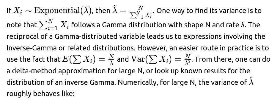
[ \huge \text{Var}(\hat{\lambda}) \approx \frac{N}{\left(\sum X_i\right)^2} \cdot \frac{1}{\lambda^2} \quad (\text{using approximate approaches}), ]
but more precise closed-form expressions exist when you incorporate the full distribution of the sum of exponentials.
How does the MLE compare to the method of moments for this parameter?

Could we use a Bayesian approach to estimate λ?

[ \huge \alpha_{\text{posterior}} = \alpha + N,\quad \beta_{\text{posterior}} = \beta + \sum_{i=1}^N x_i. ]

Are there any edge cases where the MLE might fail?

How can we check the fit of the exponential model?
Goodness-of-fit tests (e.g., Kolmogorov–Smirnov test): Compare empirical distribution with the theoretical exponential distribution.
Q-Q plots or P-P plots: Plot the empirical quantiles against theoretical exponential quantiles.
Residual analysis: Look at the pattern of residuals after fitting; if it departs significantly from what we expect, the model might be inadequate.
All of these checks help confirm whether the exponential assumption is consistent with the observed data.
Practical tips for implementation in Python
Below is a simple illustration of how you might compute the MLE in Python, given an array of sample values stored in data:
import numpy as np

def mle_exponential(data):
    """
    Computes the MLE for the rate parameter of the exponential distribution.
    data: an array or list of i.i.d. exponential samples.
    Returns: MLE for λ.
    """
    n = len(data)
    if n == 0:
        raise ValueError("No data provided.")
    if any(x < 0 for x in data):
        raise ValueError("Exponential data must be non-negative.")
    return n / np.sum(data)

# Example usage:
sample_data = [0.2, 0.5, 0.3, 1.2, 0.8]
lambda_hat = mle_exponential(sample_data)
print("Estimated rate parameter λ:", lambda_hat)
This snippet checks a few potential issues (like empty data or negative values) and returns the MLE for λ as derived.
Below are additional follow-up questions
What if we consider Maximum A Posteriori (MAP) estimation instead of MLE for λ?
A MAP estimation approach incorporates a prior belief about λ. For an exponential distribution, a common choice is a Gamma prior because it is conjugate. If we denote this prior as Gamma(α, β), meaning its PDF is proportional to:

The difference is driven by the prior parameters (α, β). When α=1 and β=0, we effectively recover the MLE. In practical scenarios, MAP can help regularize the estimate, especially when the dataset is small or we have strong reason to believe λ should stay in a certain range. A typical pitfall is selecting a prior that is too narrow, which might bias the estimate if the prior is inconsistent with the actual data.
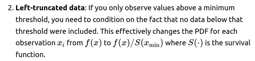
How does censored or truncated data affect the estimation of λ?
In real-world studies, it is not uncommon to encounter censored or truncated datasets. Censoring arises when some event times are only partially observed (e.g., you only know that an event time exceeded a certain threshold but not the actual time). Truncation might happen when events below or above a certain threshold are excluded from the study entirely.
Right-censored data: Suppose we know that some observations are “at least T” but the exact time is unknown. In that case, the likelihood contribution for a censored observation is the survival function S(T)=exp(−λT) for the exponential distribution. This modifies the total likelihood, which is now a product of “full likelihoods” for the uncensored data points (as before) and “survival function terms” for the censored points.

Estimation then proceeds via maximizing this adjusted likelihood that accounts for the known partial information. A common pitfall is to proceed with a standard MLE formula without considering censored or truncated observations, which can seriously bias the estimate of λ. Proper handling often requires iterative procedures (e.g., the EM algorithm) to incorporate the partially known information.
What happens if the data might come from a mixture of exponentials?

where each component has weight πₖ and rate λₖ. Estimating these parameters usually involves an EM algorithm because there is a latent label (which component each sample belongs to). One subtle pitfall is that if a single exponential assumption is forced, the MLE can systematically under or overestimate λ. You also have to check for identifiability: with multiple components, the number of parameters grows, so you need enough data to avoid degeneracies (where multiple solutions to the likelihood can appear).
Are there alternative robust estimators for λ in the presence of outliers?
While the exponential distribution technically does not have a “heavy tail” (in the sense that a single outlier should not create an infinite mean), occasionally measurement errors or extreme events can inflate the sample mean. One might consider robust estimators that down-weight extreme observations. For instance:
Trimmed means: Ignoring or trimming the largest 1–5% of data points and then inverting the resulting mean can reduce the influence of outliers.
Winsorized estimators: You replace extreme values beyond certain percentiles with the percentile boundaries, effectively capping them.
M-estimators: In principle, you could define an M-estimator for the exponential’s rate parameter that penalizes very large residuals.
However, each robust approach modifies the pure MLE and might introduce bias. A major pitfall is that if the outliers are genuine (not errors), discarding them can lose crucial information about the true distribution. The best practice is to investigate whether the “outliers” represent actual rare events or simple measurement errors.
How do we handle numerical underflow or overflow issues when computing the likelihood for large sample sizes?

A subtle pitfall occurs when you rely on direct floating-point exponentiation for extremely large or small exponents. This can crash or produce NaNs. Using log-sum-exp transformations or specialized numerical libraries can circumvent this.
How do we address a scale parameterization rather than a rate parameterization?

Would applying a logarithmic transform to the data help diagnose departures from an exponential assumption?
A typical property of the exponential distribution is that X is memoryless and that log(X) might not have a simple distribution (unlike a lognormal, for instance). One approach to diagnosing exponential fit is to look at the “exponential probability plot.” Another approach involves looking at whether −log(1−F(x)) forms a straight line with respect to x, where F(x) is the empirical cumulative distribution function. If the relationship deviates significantly from linearity, that indicates the data may not be well-fit by an exponential.
A log transform of the raw data, log(X), can highlight heavier-tailed or lighter-tailed behaviors than the exponential assumption. If the distribution of log(X) shows a strong skew or curvature in a Q–Q plot against a theoretical distribution, then the exponential might not be the right model. One pitfall is that a single large outlier can also cause spurious patterns in these diagnostic plots, so interpret them carefully.
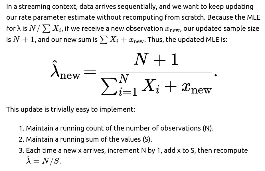
How would you update the MLE for λ in an online or streaming setting?

A subtlety in streaming applications is whether the underlying process might change over time (non-stationarity). If the process’s rate parameter shifts, older data might no longer reflect the new regime. In that case, a rolling or exponentially weighted version of the sums could be used to give more weight to recent data. But this is no longer the pure MLE under stationary assumptions; it’s a pragmatic approach for evolving processes.