ML Interview Q Series: Estimating True Classifier Accuracy Using Confidence Intervals Based on Test Set Performance.

📚 Browse the full ML Interview series here.

Confidence Interval for Model Accuracy: After training a classifier, you find its accuracy on a test set is 80% based on 1000 samples. How could you compute a 95% confidence interval for the true accuracy of the model on the population? *Explain what this confidence interval means and why it might be more informative than just the point estimate of 80%.*

Detailed Explanation of Confidence Intervals for Model Accuracy

Overview of the Core Idea Confidence intervals for classification accuracy (or any other performance metric that can be treated as a proportion) provide a range of plausible values for the true performance of a model on the broader population. In this case, we have 1000 samples in a test set and observe 80% accuracy. This 80% is called a point estimate for the true underlying accuracy. Because of sampling variability and uncertainty about whether the test set is perfectly representative of the broader population, it can be very useful to construct an interval around the point estimate. That interval is typically referred to as a confidence interval in frequentist statistics.

Understanding the Terminology of "True Accuracy" The term "true accuracy" refers to the performance a model would achieve on the entire population of interest if we had infinite data under exactly the same conditions as those in which we tested. Because we only have a finite sample of 1000 test points, we can only estimate that performance. The confidence interval quantifies the uncertainty around that estimate by providing lower and upper bounds that the true accuracy is likely to fall within, given a specified confidence level, most commonly 95%.

Confidence Interval Computation (Normal Approximation Approach) One standard way to construct a 95% confidence interval for the accuracy (or any binomial proportion) is to treat accuracy as a proportion of successes (in our example, correct classifications) over the total number of trials (test samples). Let the observed accuracy be denoted as

Detailed Explanation of Confidence Intervals for Model Accuracy

Overview of the Core Idea Confidence intervals for classification accuracy (or any other performance metric that can be treated as a proportion) provide a range of plausible values for the true performance of a model on the broader population. In this case, we have 1000 samples in a test set and observe 80% accuracy. This 80% is called a point estimate for the true underlying accuracy. Because of sampling variability and uncertainty about whether the test set is perfectly representative of the broader population, it can be very useful to construct an interval around the point estimate. That interval is typically referred to as a confidence interval in frequentist statistics.

Understanding the Terminology of "True Accuracy" The term "true accuracy" refers to the performance a model would achieve on the entire population of interest if we had infinite data under exactly the same conditions as those in which we tested. Because we only have a finite sample of 1000 test points, we can only estimate that performance. The confidence interval quantifies the uncertainty around that estimate by providing lower and upper bounds that the true accuracy is likely to fall within, given a specified confidence level, most commonly 95%.

Confidence Interval Computation (Normal Approximation Approach) One standard way to construct a 95% confidence interval for the accuracy (or any binomial proportion) is to treat accuracy as a proportion of successes (in our example, correct classifications) over the total number of trials (test samples). Let the observed accuracy be denoted as

and the sample size be

n=1000.

When the sample size is large enough for the normal approximation to be reasonable (often a rough rule of thumb is that both ( n \hat{p} ) and ( n (1 - \hat{p}) ) exceed 5 or 10), we can approximate the distribution of

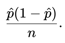
by a normal distribution centered at (\hat{p}) with variance

At a confidence level of 95%, the critical value from the standard normal distribution is often denoted as

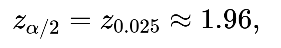
where (\alpha = 1 - 0.95 = 0.05). Hence, a typical 95% confidence interval for the proportion is

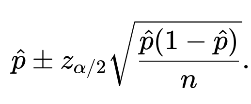
Substituting (\hat{p} = 0.8) and (n = 1000) into the formula:

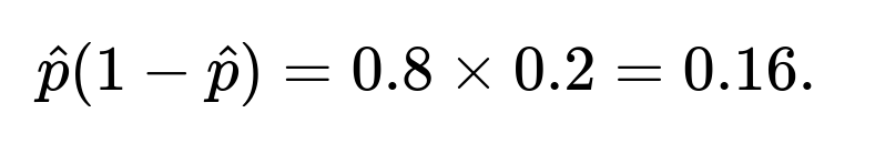
The standard error is

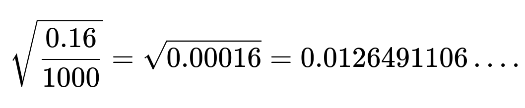
Hence the margin of error (the half-width of the interval) is approximately

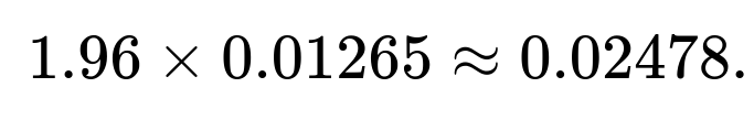
Therefore, the 95% confidence interval is approximately

0.8±0.02478,

which translates to roughly [0.7752, 0.8248], or about [77.52%, 82.48%].

Illustration in Python

import math

p_hat = 0.8
n = 1000
z = 1.96  # Approx for 95% confidence
standard_error = math.sqrt((p_hat * (1 - p_hat)) / n)
margin_of_error = z * standard_error
lower_bound = p_hat - margin_of_error
upper_bound = p_hat + margin_of_error

print(f"95% Confidence Interval: [{lower_bound:.4f}, {upper_bound:.4f}]")

Alternative Methods (Exact and Bootstrap) There are alternative approaches for constructing confidence intervals for a proportion or accuracy measure. One popular choice is the Clopper-Pearson interval, which is considered an exact method based on the Binomial distribution rather than relying on the normal approximation. Another approach is the Wilson interval, which often yields more accurate coverage for proportions close to 0 or 1. A practical, empirical approach involves bootstrapping by resampling (with replacement) from the original set of predictions and computing accuracies for many resampled datasets. Each approach has its own set of advantages and limitations. In practice, when (n) is large and (\hat{p}) is not too close to 0 or 1, the simpler normal approximation interval is often acceptable.

Interpretation of This Confidence Interval If someone repeats the entire process of data collection and computing an accuracy estimate (under the same conditions) many times, 95% of those calculated confidence intervals (constructed in the exact same way) would contain the true underlying accuracy. It is not correct to say that the probability is 95% that the true accuracy lies in any given interval—this is a subtle but important distinction in frequentist statistics. Nevertheless, it still provides a practical sense of how stable or variable that 80% figure is likely to be, under repeated sampling.

Why It Is More Informative Than Just a Point Estimate A single number like 80% doesn't capture the range of plausible values for how well the model might perform more generally. That single figure can be misleading if the test set was small or if it had particular characteristics that deviate from the broader distribution of real-world scenarios. The confidence interval offers additional context. If the interval is wide, it indicates that one should be less certain about the precision of the model's performance estimate. If the interval is very narrow, it suggests that the performance is measured with high precision given the test set size. This contextual information is critical for decision-making processes, particularly when business or safety concerns demand an understanding of how reliable or variable the model's performance could be.

Potential Pitfalls One subtle pitfall is that this interval addresses random variation in sampling the test set only. If the model or data generation mechanism changes over time, or if the data distribution in real-world deployment differs substantially from what was used to produce the test set, this confidence interval might not reflect the actual real-world performance. Another potential pitfall is misunderstanding the interval's meaning by concluding that there is a 95% probability that the true accuracy is in that interval. The frequentist interpretation is slightly different: the procedure of constructing intervals at the 95% level will capture the true parameter 95% of the time, but it is not strictly about the probability that any specific computed interval contains the true value.

Examples of When This Matters in Practice It can be critically important in scenarios where high-stakes decisions are based on model predictions. For example, in medical diagnosis, if a model is said to be 80% accurate, decision makers should also know that it could be slightly lower or higher depending on how the sample was drawn. The confidence interval might show it is plausible that accuracy is below the 78% mark or above 82%, which might influence policies, resource allocation, or further validation efforts.

Practical Implementation Advice When computing confidence intervals for accuracy or any other performance measure, always ensure that the sample size is large enough and that the distribution of classes in the test set reflects the real-world distribution. If your class distribution is different from real-world prevalence, your accuracy might not generalize. In such cases, consider approaches like stratified sampling or evaluating performance metrics more robust to class imbalance (precision, recall, F1-score). The confidence interval approach can be similarly applied to other metrics, but additional care is required if the distribution of the metric is not binomial (for instance, for continuous-valued metrics like mean squared error, we need different frameworks).

How could we interpret the lower and upper bounds in practical terms?

If the lower bound is approximately 77.5% and the upper bound is approximately 82.5%, it suggests that, based on our sample of 1000, we are fairly confident that the true accuracy of the model in the broader population would not be less than 77.5% and not more than 82.5% (in the frequentist sense). If the interval is too wide for practical purposes, that might prompt seeking more data or refining the model.

In what situations would we need to use an exact interval instead of a normal approximation?

When ( n \hat{p} ) or ( n (1 - \hat{p}) ) is small, the normal approximation can be quite poor. Also, if the accuracy is extremely high or extremely low (close to 1 or 0), the actual distribution of the estimator can deviate significantly from the normal approximation. In such cases, the Clopper-Pearson interval or the Wilson interval often provides more accurate coverage. The normal approximation can give intervals that might go below 0% or above 100% in extreme cases, which is nonsensical for an accuracy measure. Exact intervals avoid that potential issue.

How does bootstrapping compare to the normal approximation?

Bootstrapping involves drawing repeated samples (with replacement) from the original test set predictions. Each resampled dataset has the same size (n), and we compute the accuracy for each resample. By taking percentiles (often the 2.5th and 97.5th percentiles) of the bootstrapped accuracies, we can approximate a 95% confidence interval. This method makes fewer theoretical assumptions (it relies on the distribution of data in the original sample) and can be more robust when distributional assumptions are questionable. However, if the original sample is not sufficiently representative, the bootstrap can replicate biases present in the original data.

Could you discuss how sample size influences the width of the confidence interval?

The formula shows that the standard error scales with ( \frac{1}{\sqrt{n}} ). That means that as (n) increases, the confidence interval tends to shrink. Hence, to achieve a narrower confidence interval (for a given confidence level), one can increase the number of test samples. For example, if you used only 100 samples with 80% accuracy, the confidence interval would be much wider, reflecting the higher uncertainty. In real-world scenarios, data collection might be expensive or slow, so there is always a balance between the cost of more data and the desired precision for your performance estimates.

Follow-up Questions and Deep-Dive Explanations

Can you explain the difference between confidence intervals and credible intervals in more detail?

Confidence intervals (CI) come from the frequentist school of statistics, where parameters are treated as fixed but unknown quantities, and the variability is due to the randomness in the sampled data. A 95% confidence interval is constructed by a procedure that, if repeated infinitely many times, would capture the true parameter 95% of the time. It is not strictly correct to say “there is a 95% probability the true value lies in this interval,” because in frequentist terms, the true parameter is fixed and does not have a probability distribution.

Credible intervals (CrI), on the other hand, come from the Bayesian school of statistics, which treats parameters as random variables with a prior distribution. After observing data, one obtains a posterior distribution over those parameters. A 95% credible interval is any interval in the posterior distribution that contains 95% of the posterior probability mass. It can be interpreted as “there is a 95% probability that the true parameter lies in this interval,” which is conceptually different from how confidence intervals are interpreted.

For a machine learning practitioner, the essential distinction is that credible intervals allow for a probabilistic statement about the parameter itself, whereas confidence intervals describe the long-run behavior of the interval construction procedure. In practical model evaluation, both intervals aim to express uncertainty about an estimate, but the philosophical underpinnings and interpretations differ. Some modern workflows use Bayesian methods to produce credible intervals for model accuracy, especially when interpretability of probability statements about parameters is crucial.

If the distribution of data changes over time, how does that affect the reliability of a confidence interval computed from older data?

If the distribution changes due to concept drift or shifts in how data is collected, the test data from the past may no longer be representative of the new conditions. A confidence interval computed from older data assumes that the distribution from which the test data was drawn remains stable. When the distribution changes, the “true accuracy” with respect to the old distribution may not match the model’s real-world performance on the new distribution.

In these scenarios, relying on an older confidence interval can lead to overconfidence or underconfidence. If the model remains the same, but the data shift significantly, you might find that your point estimate of accuracy changes, and the historical confidence interval no longer accurately reflects uncertainty about the new accuracy. One practical approach is continuous monitoring of the model’s performance on recent data and recalculating or updating confidence intervals accordingly. Another approach is using domain adaptation techniques or re-training the model when distribution shifts occur. The main point is that a confidence interval’s validity depends on the assumption that the data generating process remains consistent. If it does not, re-computation is essential.

Could you discuss the Wilson interval in more detail and how it differs from the standard normal approximation?

The Wilson interval is an alternative to the standard normal approximation for constructing confidence intervals of a binomial proportion. It is often given by a formula that avoids some of the less desirable properties of the naive normal approximation. The normal approximation can yield intervals that go below 0 or above 1, especially when (\hat{p}) is near 0 or 1 or (n) is not large. The Wilson interval typically remains within [0, 1] and can produce more accurate coverage probabilities even for moderately sized samples.

In practice, the Wilson interval for a proportion can be written in a form that, instead of centering around (\hat{p}), centers around a slightly adjusted value. It also adjusts the standard error in such a way that leads to intervals that are more stable. The formula for the Wilson interval can be found in many references, and it often yields good coverage properties regardless of whether ( n\hat{p} ) and ( n(1-\hat{p}) ) are large enough. Many statistical software libraries (for example, statsmodels in Python) provide a direct function to compute the Wilson interval. In many real-world analyses, especially when the sample size is not extremely large, the Wilson interval is considered a better default choice than the simple normal approximation.

The difference between them is mostly in how the interval is derived. The Wilson approach re-centers and re-scales the proportion in a manner that better matches the true binomial distribution. In contrast, the naive approach tries to approximate the binomial distribution with a normal distribution that might not accurately reflect small sample sizes or extreme proportions.

When deciding which interval to use, many statisticians recommend the Wilson interval or a related approach such as the Agresti-Coull interval over the plain normal approximation. But for large ( n) and not-too-extreme values of (\hat{p}), they will be very similar to one another in practice.

---

Below are additional follow-up questions

How would you handle constructing confidence intervals for accuracy in a multi-class classification setting?

When dealing with multi-class classification, accuracy is still the ratio of correctly classified samples to the total number of samples, but there are multiple classes rather than just two. The simplest extension of the binomial-based confidence interval for accuracy in a multi-class problem treats each prediction as either correct or incorrect, effectively reducing the outcome to a binary event of "correct vs. incorrect." Once you do this reduction, you have a proportion of correct classifications (still (\hat{p} = \frac{\text{number of correct predictions}}{n})), and you can apply the same binomial-based formula (normal approximation, Wilson, Clopper-Pearson, bootstrap, etc.) to derive a confidence interval for the overall accuracy.

A deeper complexity arises when you also want per-class accuracy. In that situation, you effectively have separate "binomial processes," one for each class (i.e., correct or incorrect predictions of that class among the samples truly belonging to that class). You could then compute a separate confidence interval for each class's accuracy. However, be mindful of these points:

• Some classes may have very few samples, making the normal approximation less reliable. Methods such as the Clopper-Pearson interval or the Wilson interval might be preferable for those lower-frequency classes.

• If the class distribution is heavily skewed, the overall accuracy might be dominated by majority classes, and the intervals for minority classes may be very wide or less meaningful without additional context or rebalancing.

• If multiple comparisons are made (e.g., you compute intervals for 10 classes), the chance that at least one of the intervals does not contain its true parameter grows if you interpret them in a purely frequentist sense. Consider adjustments for multiple testing if you want strong statements across multiple intervals simultaneously.

Pitfalls and Edge Cases

• Using overall accuracy alone in a highly imbalanced multi-class problem can be misleading, even if it has a narrow confidence interval. A scenario with a dominant class can yield a deceptively high accuracy but poor performance on other classes.

• If your test samples are correlated or come from a sequence, the binomial assumption of independence might be violated, leading to intervals that are too narrow.

• If class definitions overlap or are fuzzy (common in multi-label scenarios), an accuracy-based confidence interval might not capture the full extent of performance.

How should confidence intervals be adjusted when test data samples are correlated or non-i.i.d.?

Many standard confidence interval methods assume that each sample is an independent Bernoulli trial. In real-world scenarios, data can be correlated in multiple ways. For instance, time-series data may have temporal correlation; images from the same scene may be correlated; data points could be nested in groups (e.g., patients within the same hospital).

When independence is violated, the simple binomial variance (\hat{p}(1 - \hat{p})/n) might underestimate or overestimate the actual variance. The usual confidence interval formulas then become unreliable.

Ways to Address Correlation

• Block Bootstrapping or Cluster Bootstrapping: Instead of sampling individual data points, sample entire correlated blocks or clusters as units. This preserves the correlation structure within each block.

• Generalized Estimating Equations (GEE): In biostatistics and related fields, GEE can be used to estimate a population-level proportion while accounting for within-group correlation.

• Variance Inflation Factors: If you know or can estimate the intra-class correlation (ICC), you can inflate the standard error to reflect the correlation. The effective sample size might be smaller than the raw (n).

Pitfalls and Edge Cases

• Ignoring correlation can lead to overly tight intervals, giving a false sense of certainty.

• Accurately estimating correlation structures can be difficult if data collection processes are complex.

• Overcorrecting for correlation can make the intervals too wide, especially if you do not have enough data to precisely estimate the correlation.

What considerations arise for constructing confidence intervals in situations with severe class imbalance?

In severely imbalanced classification tasks, the overall accuracy might be extremely high simply by predicting the majority class most of the time. Constructing a confidence interval around that high accuracy does not necessarily highlight the model’s performance on rare classes. Key points to consider:

1. Stratified Sampling: Ensuring your test set has adequate representation of each class can help you compute more reliable estimates of performance.

2. Precision, Recall, F1-score: Sometimes, accuracy confidence intervals are less informative if most samples belong to a single class. Confidence intervals for metrics such as precision or recall on the minority class might be more meaningful.

3. Separate Interval per Class: You might construct a separate binomial confidence interval for the accuracy on each class, or for key metrics like recall for the minority class.

Pitfalls and Edge Cases

• A tight interval around a high accuracy in an imbalanced scenario can be misleading if the minority class has minimal support.

• If the minority class frequency is very small, the normal approximation will be especially suspect. Consider using an exact method like Clopper-Pearson or a Bayesian approach.

• If your test set is large enough overall but still yields very few minority samples, the interval for minority class accuracy could be very wide. This might be hidden by just quoting the overall accuracy interval.

Are there distribution-free methods to construct a confidence interval for accuracy?

Yes, one common distribution-free approach is the bootstrap, where you do not explicitly assume a binomial or normal distribution but rely on random resampling from the empirical distribution of (prediction, ground-truth) pairs:

• Non-Parametric Bootstrap: Repeatedly resample your test set with replacement, compute the accuracy on each resampled set, and then take (for a 95% CI) the 2.5th and 97.5th percentiles of those accuracy values. This gives you an empirical interval based solely on your observed data.

• Permutation Tests: For certain hypothesis testing frameworks, one might do a permutation-based approach to measure how accuracy changes under random label permutations. However, this is more for significance testing than a straightforward confidence interval.

Pitfalls and Edge Cases

• If the test set is small or unrepresentative, bootstrapping might amplify biases present in the original sample.

• Highly correlated data can render bootstrap samples less varied than you might assume. Adjustments like moving block bootstrap or cluster bootstrap may be needed.

• Bootstrapping can be computationally expensive for large-scale models, though in practice, it’s often feasible with careful coding or parallelization.

How could prior knowledge be incorporated to refine interval estimates for accuracy?

In a Bayesian framework, you can place a prior distribution on the true accuracy (p). After observing your test data (e.g., (k) correct out of (n)), you update this prior to a posterior distribution using Bayes’ rule. The posterior distribution for (p) will then be used to derive a credible interval rather than a confidence interval. This can be particularly helpful if:

• You have strong domain knowledge suggesting the accuracy should be near a certain range.

• You have historical data from similar tasks or previous model versions that might inform a prior distribution for performance.

Pitfalls and Edge Cases

• If the prior is too strong (i.e., highly concentrated in a small region), it might dominate the posterior, ignoring the observed data.

• If the prior is poorly chosen (not informed by real-world considerations), the resulting credible interval might be misleading.

• Switching between frequentist and Bayesian interpretations can confuse stakeholders who are used to traditional confidence intervals.

What are the trade-offs between using a single hold-out test set vs. cross-validation for constructing confidence intervals?

1. Single Hold-out

   • Simpler conceptual approach: train once, test once, compute the binomial proportion for accuracy.

   • Confidence intervals are straightforward to compute but reflect only one particular split of train/test.

   • If (n) is not large, the variance in the estimate can be quite high and might not generalize well to unseen data splits.

2. Cross-Validation

   • Repeatedly splitting data into training and validation folds provides multiple estimates of accuracy.

   • The distribution of these estimates can be used to construct a confidence interval (e.g., by looking at the mean and standard deviation of the cross-validation accuracies).

   • More computationally expensive, but typically more reliable and robust, especially for smaller datasets.

Pitfalls and Edge Cases

• If data has temporal or grouped structure, standard cross-validation might break these correlations, leading to overly optimistic intervals.

• Variance estimates from cross-validation can be tricky because the folds are not entirely independent. Methods like repeated cross-validation or nested cross-validation can help but are even more computationally expensive.

• Using cross-validation intervals for final model performance might differ from intervals using a strictly unseen hold-out set. Practitioners often prefer a separate, final hold-out set for a last unbiased performance check.

How does repeated or nested cross-validation influence confidence intervals for accuracy?

Repeated Cross-Validation: You repeatedly perform something like 5-fold or 10-fold cross-validation multiple times with different random splits. This yields multiple accuracy estimates. One can then calculate the mean and standard deviation across all these runs, forming the basis for a confidence interval (often using a t-distribution if the sample of accuracy estimates is not large).

Nested Cross-Validation: Typically used when you want both model selection (hyperparameter tuning) and performance estimation in a principled way. In each outer fold, you train a model (which inside that fold may itself use cross-validation for tuning) and then evaluate on the held-out portion of data. You then average the outer-fold performance results for an unbiased performance estimate.

Pitfalls and Edge Cases

• The estimates from repeated cross-validation are not entirely independent, so standard formula-based intervals can be too narrow. More sophisticated methods might be needed.

• If the data is not large, repeated cross-validation might lead to training sets that overlap heavily, creating correlated performance estimates.

• Nested cross-validation is computationally intensive. You must weigh the benefits of a robust, unbiased estimate with the cost in runtime, especially for large models.

In high-availability industrial systems with continuous data ingestion, how do you maintain and interpret a confidence interval for accuracy over time?

In practice, models often receive a continuous stream of new data. Your original confidence interval might become stale if the data distribution shifts. Approaches to maintain a current confidence interval include:

1. Rolling Windows: Keep a sliding window of the most recent data (e.g., last 10,000 samples). Continually re-estimate accuracy and update the interval. This ensures the interval reflects current conditions but might lose historical context.

2. Exponential Decay Weighting: Weight more recent samples higher and older samples lower, so the estimate focuses on recent performance trends.

3. Online Learning or Online Evaluation: If the model updates in an online fashion, pair it with an online estimation of performance variability.

Pitfalls and Edge Cases

• Concept drift can make older performance data irrelevant. A stable, narrow confidence interval that does not adapt to drift is misleading.

• Data quantity at each time slice might vary, causing intervals to widen or narrow unexpectedly if there are fluctuations in data flow.

• Implementation complexity: constant recalculation of intervals requires good engineering practices to ensure correctness and efficiency in streaming environments.

How do we statistically compare two models’ accuracy intervals to see if one model is significantly better?

If you have two models, each with an estimated accuracy from the same test set, you can compare them in a few ways:

1. Confidence Interval Overlap: A naive approach is to see if the intervals for the two accuracies overlap. However, if intervals do not overlap, you can be more certain one model is better, but overlapping intervals does not necessarily mean there is no significant difference (they can overlap and yet there could still be a statistically significant difference).

2. McNemar’s Test: Common for comparing two classifiers on paired data (same test set). It focuses on the disagreements where one model is correct and the other is incorrect.

3. Bootstrap-based Comparison: Resample the test data with replacement, compute the accuracy difference for each bootstrap sample, and get a confidence interval for the difference. If the interval does not contain zero, that indicates a significant difference at the chosen confidence level.

Pitfalls and Edge Cases

• If the test sets are different for each model (e.g., each model was tested at a different time), the comparisons might not reflect the same data distribution.

• If the models were tuned extensively on the same test set, the test set might become a biased measure.

• McNemar’s test specifically looks at the number of test instances for which models disagree; if that number is small or the data set is small, the result might be unreliable.

When is it appropriate to aggregate multiple test sets into one bigger set for a single confidence interval, and what can go wrong?

Sometimes practitioners have multiple smaller test sets collected at different times or from different sources. They might want to combine them into one larger set to get a narrower confidence interval. This can be valid if:

• The test sets come from the same distribution.

• There is no time-based or domain-based shift that would cause the sets to reflect different populations.

• The samples are treated as if i.i.d. when pooled together.

Potential Pitfalls

• If the test sets differ systematically (e.g., one set is from older data, another from a new population), the combined set might not represent any single real-world distribution well.

• If correlation exists within each subset or across them, the usual binomial formula might underestimate variance.

• If you merge sets with widely varying class distributions, the combined accuracy might become a mixture that doesn’t reflect performance on any specific distribution well.

What if the test set contains uncertain or “soft” labels rather than definitive ground-truth labels?

In some domains, labels might be probabilistic or “soft,” reflecting uncertainty (e.g., medical diagnoses that are not 100% certain). The notion of “accuracy” becomes more complicated because each label is not simply correct or incorrect. Approaches include:

• Thresholding the Soft Labels: Convert them to hard labels at a certain probability threshold. But this can introduce subjectivity, and the resulting binomial intervals might not reflect the label uncertainty.

• Scoring Rules: Instead of measuring accuracy, consider a proper scoring rule (like log loss or Brier score) and then construct intervals for that.

• Bayesian Label Model: If you treat each label as drawn from a latent ground truth distribution, you could estimate the posterior of the model’s performance given these uncertain labels.

Pitfalls and Edge Cases

• Hardening the labels too early can hide the labeler’s uncertainty.

• If the labeling process is itself noisy or biased, your intervals for accuracy can be systematically shifted.

• Inter-annotator variability can cause wide discrepancies in how “soft” is defined or measured.

How do we construct a confidence interval for metrics like AUC or log loss, which are not simple binomial proportions?

For metrics such as the Area Under the ROC Curve (AUC) or log loss, the underlying distribution is not binomial, so the standard (\hat{p} \pm z_{\alpha/2}\sqrt{\hat{p}(1-\hat{p})/n}) formula does not apply directly. Some methods:

1. DeLong’s Method: Specifically for the AUC, DeLong’s test or variance estimation is a nonparametric approach that can provide confidence intervals for AUC.

2. Bootstrap: A more general approach is to bootstrap the test set, compute the AUC or log loss for each resample, and use percentiles of the bootstrap distribution to form an interval. This method is flexible and widely used in practice.

3. Asymptotic Approximations: In large samples, you might approximate the variance of the AUC or log loss, but the formula is more involved than the binomial proportion.

Pitfalls and Edge Cases

• The reliability of DeLong’s method depends on how well the test data represents the score distributions.

• For log loss or other continuous metrics, you might have outliers that cause large variance and thus wide intervals.

• Bootstrapping can be computationally expensive if your dataset is large and your model is costly to evaluate many times.

What role do sampling strategies (like stratified or cluster sampling) play in confidence interval calculations for accuracy?

Stratified Sampling

• If your dataset is stratified to reflect class proportions, your estimate of accuracy will be more stable, especially for minority classes.

• If your actual real-world distribution differs from the stratified distribution in the test set, your intervals might not reflect the real world accurately. You would need to re-weight or post-stratify your estimates.

• Confidence intervals might be narrower because stratification reduces variance, but that assumes you are truly capturing real-world class ratios or adjusting accordingly.

Cluster Sampling

• If data is sampled by cluster (e.g., by geographic region, hospital, user group), the independence assumption can be violated within each cluster.

• Typically, you would account for the design effect or cluster effect in the variance estimate. Failing to do so might yield over-confident intervals.

• If cluster sizes vary widely, special care is needed in how you weight the clusters when constructing an overall accuracy and its confidence interval.

Pitfalls and Edge Cases

• Failing to incorporate the sampling design in the variance calculation can produce intervals that are biased or too narrow.

• Overly complex sampling designs (like multistage sampling) might require specialized survey methods or weighting to get correct intervals.

• If the real deployment scenario does not match the sampling design, interpretation of the intervals might be off in practice.

How should we handle multiple comparisons when evaluating accuracy across many models or hyperparameter configurations?

If you train many different models or tune hyperparameters extensively, you might end up with multiple accuracy estimates—one for each model or setting. Constructing separate confidence intervals for each one can inflate the chance of incorrectly concluding that a model is significantly better than others if you do not correct for multiple testing. Options include:

• Bonferroni Correction: Adjust the significance level by dividing by the number of comparisons, though this can be conservative and lead to wide intervals.

• Holm-Bonferroni or Benjamini-Hochberg: More nuanced procedures for controlling family-wise error or false discovery rates.

• Cross-Validation with Statistical Tests: Use repeated cross-validation and pairwise tests, applying multiple comparison adjustments to the p-values.

Pitfalls and Edge Cases

• Over-optimizing hyperparameters on the test set effectively contaminates the test set. This leads to intervals that do not reflect unbiased performance.

• Large-scale hyperparameter searches with random seeds can produce many accuracy values, some of which might appear high purely by chance.

• Very large corrections (e.g., Bonferroni) might make it hard to claim significance for any difference, even if practical differences exist.

How might domain-specific constraints or performance thresholds affect the interpretation of accuracy confidence intervals?

Certain domains have strict performance needs—e.g., a medical device might need at least 90% accuracy to be considered for regulatory approval. If your 95% confidence interval is [88%, 92%], from a purely statistical standpoint you can say the model might or might not meet the 90% threshold. But domain-specific constraints often dictate:

• Regulatory Requirements: You might need an interval that reliably exceeds a threshold, not just an interval that contains it.

• Safety Margins: In safety-critical systems, you might want a 99% confidence interval or a lower bound that comfortably clears a necessary threshold for reliability.

• Risk Tolerance: If a misclassification is extremely costly, your domain might require a narrower confidence interval or a higher confidence level (e.g., 99.9%) to ensure performance is sufficiently proven.

Pitfalls and Edge Cases

• Overly strict thresholds combined with wide intervals can render an otherwise high-performing model unacceptable for deployment.

• Real-world distribution changes might invalidate your intervals, so you cannot claim domain compliance if the data environment shifts.

• In some domains, accuracy alone might be insufficient if certain classes carry dramatically higher risk when misclassified.

Could you describe practical scenarios where a confidence interval for accuracy is insufficient on its own?

While confidence intervals for accuracy are important, certain real-world scenarios demand additional or alternative analyses:

1. High-Risk Applications: In autonomous vehicles, aviation, or medical interventions, you may need reliability measures that exceed typical 95% confidence intervals, or you might focus on worst-case scenarios (e.g., guaranteeing no more than 1 misclassification in 1000 for a certain condition).

2. Explainability or Accountability: Some contexts require understanding why errors occur. A single interval for accuracy does not explain which subpopulation or scenario is causing failures.

3. Continuous Deployment: If the model is updated weekly, you might need a robust mechanism for tracking performance drift and re-validating intervals frequently.

4. Cost-Sensitive or Utility-Based Settings: Accuracy might not reflect the true cost or utility. For example, in fraud detection, a single missed fraudulent case could be extremely costly, so you might rely more on recall or precision in the minority class.

Pitfalls and Edge Cases

• Focusing solely on an accuracy interval can lead to neglect of model biases or ethical concerns in certain subgroups.

• In large-scale systems, an accuracy interval might be narrow, yet small error rates can still affect thousands or millions of users, so operational risk can be significant.

• Some domains measure success not by raw accuracy but by cost savings, revenue impact, or user satisfaction, requiring different metrics and intervals.

How can domain knowledge be leveraged to refine data collection and thus narrow the confidence interval for accuracy?

Domain knowledge can inform better data collection strategies, improving the representativeness and size of the test sample. A more representative and larger test sample can lead to:

• Reduced Variance: If your domain knowledge helps ensure test data covers typical real-world use cases and edge cases, the estimate of accuracy can be more robust, potentially yielding a tighter interval.

• Targeted Sampling: Collecting more samples specifically from known challenging conditions or from subpopulations underrepresented in the training data can clarify the model’s strengths and weaknesses.

• Focused Budget Allocation: Instead of randomly collecting data, domain experts can guide sampling to maximize the value of new test points, ensuring that each additional sample helps clarify performance in critical areas.

Pitfalls and Edge Cases

• Over-targeting specific scenarios can bias the distribution of the test set, inflating or deflating overall accuracy artificially.

• Relying too heavily on domain knowledge might exclude unknown novel cases.

• Domain-driven data collection might be costly or time-consuming, so practical trade-offs must be made.

How would you approach explaining these intervals and their interpretation to non-technical stakeholders?

While the mathematics behind confidence intervals can be intricate, especially in the presence of advanced methods or correlation, you can still convey the essence:

• Focus on the Range: Emphasize that “We believe the model’s accuracy on this type of data lies roughly between X% and Y%, given our current sample.”

• Probability vs. Procedure: Caution that “This does not mean there is an X% chance that the true accuracy is in this range, but rather if we repeated this testing approach many times, about 95% of the intervals computed would capture the true accuracy.”

• Implications for Risk: Translate the interval width into a statement about how stable or uncertain the model’s performance might be. A wide interval indicates “We are not fully sure how well the model performs; more data or further analysis is needed.”

• Contextualize with Business or Real-World Outcomes: For example, “If the lower bound of 78% accuracy is still acceptable for our application, we can proceed. Otherwise, we may need to gather more data or improve the model.”

Pitfalls and Edge Cases

• Non-technical audiences often interpret intervals incorrectly as “We are 95% sure that the true accuracy is in this range.” While often used colloquially, it is not strictly correct in the frequentist sense.

• If the confidence interval is small, there can still be domain drift or mismatch with real-world usage that is not captured.

• Over-simplifying or overselling the meaning of the interval can lead decision-makers to place unwarranted trust in the model’s performance.