ML Interview Q Series: Estimating Expected Wait Time for Normal Exceedance with Geometric Distribution.

Browse all the Probability Interview Questions here.
2. You are drawing from a normally distributed random variable X ~ N(0, 1) once a day. What is the approximate expected number of days until you get a value of more than 2?
This problem was asked by Quora.
To address this question, we want to find the expected waiting time (in days) until we see a draw from a standard normal distribution that exceeds 2. Below is a step-by-step reasoning process in detail:
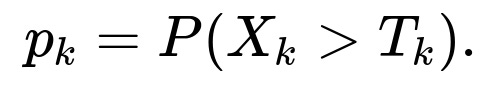
Understanding the Distribution and Probability of Exceeding 2 The random variable X is distributed as N(0,1), meaning it has mean 0 and variance 1. We are interested in the event X>2. The probability of X exceeding 2 on any single draw is:

where Φ(⋅) is the cumulative distribution function (CDF) of the standard normal distribution N(0,1). The exact value of Φ(2) is approximately 0.9772. Therefore:
Interpreting the Problem Using a Geometric Distribution Every time we draw from the distribution, we can think of it as a “trial” that either succeeds (i.e., we get X>2) with probability p≈0.0228 or fails (i.e., we get X≤2) with probability 1−p≈0.9772.
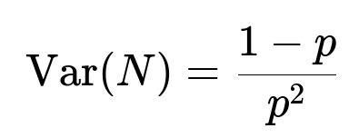
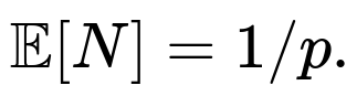
If we denote by N the (random) number of days until we get our first draw that exceeds 2, then N follows a geometric distribution with parameter p=P(X>2). Recall that if a random variable N follows a geometric distribution with parameter p, its expected value is given by:

Hence:
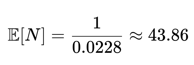
So the expected number of days until seeing a value more than 2 is approximately 44 days (some might round it to 44).
Why This Makes Sense Intuitively, the probability of exceeding 2 (which is about 2 standard deviations above the mean in a standard normal distribution) is not very high (roughly 2.28%). Hence, on average, you might need around 44 draws for one of those draws to exceed 2.
Real-World Considerations and Pitfalls
• Estimation vs. Exact Value: Since the true probability P(X>2) is about 0.0228, we are relying on the numerical value of the standard normal CDF at 2. If someone approximated P(X>2)differently (say 0.0227 or 0.0230), that would slightly change the final estimate.
• Large Number of Trials vs. Single Outcome: In reality, it’s entirely possible to draw a value more than 2 after just a few days or wait much longer than 44 days, because waiting times in a geometric scenario have a “memoryless” nature. The number 44 just represents an average.

• Potential Off-By-One Convention: Some formulations of the geometric distribution define it differently (i.e., the number of failures before the first success). Here, we interpret N as the total number of trials up to and including the success. The standard version we use here is E[N]=1/p.
Putting It All Together The approximate expected number of days is around 44. That is the short and clear answer. However, in an interview or exam, it is important to articulate all the reasoning steps, including how the probability is derived from the standard normal distribution and how that leads to the expectation of a geometric random variable.
Possible Follow-up Questions and Detailed Answers
What if we wanted the expected time until we get a value more than 2.5 instead of 2?
To find the expected number of days until X>2.5, we can follow the same steps but replace 2 with 2.5:
Calculate P(X>2.5)=1−Φ(2.5). Numerically, Φ(2.5) is about 0.9938, so:


So on average, it would take about 161 days.
In an interview, you might explain how the general formula extends to any threshold a:

You should discuss numeric approximations of Φ(a), how to calculate it programmatically (e.g., with a library like scipy.stats in Python), and note that the expected time can quickly become very large as aa grows, because P(X>a) shrinks rapidly.
How would you implement a simulation in Python to approximate this result?
Below is a simple illustrative Python code snippet. This code performs a Monte Carlo simulation to empirically estimate the number of days needed until the draw from N(0,1) is above 2.
import numpy as np

def simulate_days_until_threshold(num_simulations=1_000_000, threshold=2.0):
    # Generate random draws all at once
    # We'll attempt to see, for each simulation, how many draws
    # it takes to exceed threshold
    # However, a more direct approach is to treat each day
    # as a Bernoulli trial with success probability p = P(X > threshold).

    # First, let's estimate p using the survival function:
    p = 1 - 0.9772 if threshold == 2.0 else None
    # Or compute it precisely with a library:
    # from scipy.stats import norm
    # p = 1 - norm.cdf(threshold)

    # We'll do a geometric approach:
    # Generate geometric random variables with success probability p
    # The geometric distribution can be generated by looking at
    # how many tries until first success.

    # Using numpy: np.random.geometric(p, size=num_simulations)
    # returns number of trials until first success (draw).
    days = np.random.geometric(p, size=num_simulations)
    return days.mean()

avg_days = simulate_days_until_threshold()
print(f"Approx. average days until exceeding 2.0: {avg_days}")
Explanation of the code logic:
• We first compute p=P(X>threshold). • We use NumPy’s
np.random.geometric(p, size=num_simulations)which draws from the geometric distribution directly. • We calculate the mean of these draws to obtain the empirical average.Alternatively, you could run a daily simulation checking day by day for each simulation, but that would be less efficient. The direct geometric generation is more appropriate.
In an interview, you should mention that direct numeric simulations can help verify theoretical conclusions, though they might be computationally expensive for smaller probabilities (very large thresholds) or extremely large numbers of simulations.
Can you discuss the difference between the “memoryless” property in the exponential/geometric distributions vs. the normal distribution?
In the context of waiting times, the geometric distribution (discrete analog of the exponential distribution in continuous time) is memoryless: If we have not yet succeeded in k trials, the probability of success on the next trial is still p, independent of k. That means the distribution “resets” after each trial.
Normal distributions are not memoryless. Knowledge of previous draws from a normal distribution does not “reset” in the same sense. However, in the scenario described in this question, each day’s draw is an independent draw from N(0,1). The memoryless property we rely on is from the Bernoulli process viewpoint: each day is an independent Bernoulli “success” with probability p or “failure” with probability 1−p. This is fundamentally a consequence of repeated independent sampling from the normal distribution, not of the normal distribution itself being memoryless.
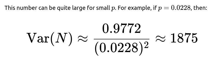
Why does the variance of the geometric waiting time matter, and what is its formula?
For a geometric random variable N with success probability p, the variance is:


Standard deviation would be 1875≈43.29, which is roughly the same order of magnitude as the mean. This indicates wide variation in possible waiting times. Some realizations might happen after just a few days, and some might take hundreds of days.
In interviews, you might be asked how you would interpret or handle such variability in practical applications—for instance, in real-world processes, having a large variance means you should plan for the possibility of either extremely early or extremely late successes.
If I only have a finite number of days, say 30 days, what is the probability that I do NOT see a value more than 2 in that time?
This question focuses on the cumulative distribution of the waiting time:

Hence:

Numerically:
import math

p = 0.0228
prob_no_exceed_2_30days = (1 - p)**30
print(prob_no_exceed_2_30days)
This follow-up question tests your ability to apply standard Bernoulli process reasoning to find probabilities of zero successes over multiple trials.
Does the Central Limit Theorem (CLT) help in any way here?
Not directly. The CLT typically tells us about the distribution of sample means (or sums) of i.i.d. random variables as the number of samples grows large. Here, we are dealing with the distribution of a single draw that might exceed some threshold, or equivalently, the waiting time until the first success. That is a different type of problem—one that is more directly described by the Bernoulli/Geometric frameworks.
A subtle confusion might arise if someone tries to apply the CLT to the maximum of i.i.d. normal draws. For large numbers of draws, the maximum eventually grows, but the result is not the same as a direct geometric waiting-time argument. Also, the extreme value distribution might come into play if one is specifically analyzing the distribution of maxima over a time window. But for the question at hand—expected days until the first exceedance—the geometric distribution approach is more straightforward.
If the distribution were not normal but some unknown distribution, how would we solve a similar problem?
The same reasoning extends:
Identify p=P(X>threshold) under the new distribution of X.
The waiting time for the first exceedance (assuming daily independent draws) is geometric with parameter p.
The expected waiting time is still 1/p.
Everything hinges on computing or estimating p=P(X>threshold). For a non-normal (possibly complicated) distribution, you might do the following in practice:
• Use empirical/historical data to estimate p (for example, count the fraction of samples that exceed the threshold). • Use a parametric or non-parametric model of the distribution and integrate its tail to find 1−F(threshold). • Use Markov Chain Monte Carlo (MCMC) methods or other sampling methods to estimate tail probabilities if the distribution is analytically difficult.
After obtaining a good estimate of p, the rest of the procedure is conceptually identical.
How do you calculate 1 - Φ(2) exactly or approximately without a standard normal table?
In modern computing environments, we typically rely on library functions such as scipy.stats.norm in Python (e.g.,
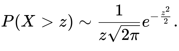
1 - norm.cdf(2)). But sometimes, interviewers might ask you to approximate 1−Φ(2) without using a direct table or library. A common approximation for the upper tail of a standard normal is given by:
for z>0. This is essentially using the asymptotic tail behavior of the normal distribution. For z=2, this yields:

This is a rough estimate (it overestimates a bit since the true value is about 0.0228). The difference arises because the integral from z to ∞ is strictly greater than just the leading term in this asymptotic approximation. Still, it is a decent quick estimate.
In an interview, if asked to do a mental approximation, you might explain or show a near approximation to 1−Φ(z) for integer or half-integer values of z using known table values or the rule-of-thumb that 1−Φ(2) is roughly 2.3%.
Are there any alternative ways to interpret or solve the problem?
One alternative perspective is that each day’s draw can be mapped to a Bernoulli trial with success probability p=0.0228. The question “expected number of days until success” is directly answered by the standard result for geometric distributions:

A purely simulation-based approach—where you literally generate day-by-day random draws from a standard normal and check how long until you exceed 2—would give a numerical estimate that converges to about 44.
Could you talk about large deviations or extreme value approaches for a bigger threshold?
If the threshold is not just 2 but some larger value (say 5 or 6) that is even rarer for N(0,1), the waiting time grows even further. One might consider large deviation principles, which say that for z large:

The event X>z becomes extremely rare, and the expected waiting time for first exceedance can become huge.

Summary
The approximate expected number of days is computed by recognizing that the event X>2 has probability 0.0228. Each day is thus a Bernoulli trial with p=0.0228. By standard geometric distribution theory, the expected number of trials (days) until the first success (exceed 2) is 1/p≈44.
This is a straightforward and common type of question that tests a candidate’s ability to (1) recall the distribution properties of the normal distribution, (2) translate a problem into Bernoulli trial language, and (3) recall or derive the expectation of a geometric random variable.
The final numeric answer to the original question is approximately 44 days.
Below are additional follow-up questions
How would the answer change if we wanted the expected number of days until we get three values above 2, rather than just one?
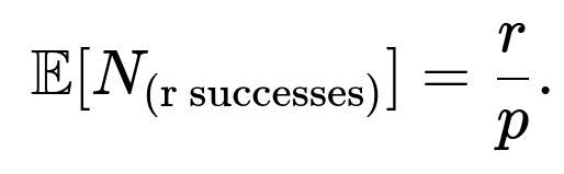
When we look for the expected number of days until we get three exceedances of 2, the situation is no longer a simple geometric distribution. Instead, we can model this as a negative binomial process where each draw is still a Bernoulli trial with success probability p≈0.0228 (the probability of exceeding 2 in a standard normal draw). The negative binomial random variable with parameters (r, p) is the count of the number of trials needed to achieve r successes, where r in this case is 3.
The expected value of a negative binomial random variable that models the number of trials needed to achieve r successes (with success probability p each trial) can be written as


In other words, on average, we would need around 132 days to get three draws exceeding 2.
Potential Pitfalls and Edge Cases • Each success event is still assumed independent. If the daily draws were correlated, this expectation would no longer hold in the same way. • We assume the standard parameterization of the negative binomial. Some texts define the negative binomial differently (e.g., modeling only the number of failures before the r-th success). • Variability can be larger when waiting for multiple successes. If we look at real data and see fewer than expected successes after many draws, we should investigate whether the assumption of independence or the distribution itself might be off.
Real-World Subtleties • In practice, if we stop early or change the threshold midstream, we break the assumption of identical Bernoulli trials. • If the probability p changes over time (due to concept drift or shift in the real-world process), we cannot simply apply the negative binomial formula.
What if we want the median number of days instead of the mean?
The original question focuses on the expected (mean) number of days. However, you might be asked for the median, which is the day ( d ) such that there is a 50% probability you have already exceeded 2 by day ( d ). For a geometric distribution with success probability p:
• The probability that you have not succeeded by day ( d ) is ( (1-p)^d ). • You want ( P(\text{No success by day } d) = 0.5 ).
Hence you solve:


So the median time is around 30 days. This is smaller than the mean (about 44 days), which is a known property of the geometric distribution: for 0 < p < 1, the mean exceeds the median.
Potential Pitfalls • Some candidates mix up the mean and median, especially under highly skewed distributions like geometric. • They might assume the median equals the mean, which is incorrect for geometric distributions. • Rounding can lead to confusion. Day 30.3 might be described as day 30 or 31 in everyday language, so clarify your rounding conventions.
Real-World Subtleties • In real operational settings (e.g., risk management), sometimes the median is more relevant than the mean if you are trying to figure out “by what day are we 50% certain to have observed an exceedance?” • The difference between mean and median waiting times can be large for very small p, so that’s important to keep in mind when setting expectations or budgets in real projects.
How would correlated daily draws affect the expected waiting time?
In the original solution, we assume each daily draw is i.i.d. from N(0,1). Now consider if there is correlation between successive daily draws (e.g., day-to-day measurements are autocorrelated). This complicates matters because the probability of success on day ( k ) might depend on whether day ( k-1 ) was above or below 2.
Even with correlation, you can still roughly estimate using the geometric approach if the correlation is modest. However, for stronger correlation, the distribution of waiting times might deviate significantly:
• If positively correlated, once we get close to the threshold on one day, the next day is more likely to also be high, so we might see clusters of exceedances. This can reduce the expected time to the first exceedance. • If negatively correlated, high draws might be followed by lower draws, which increases the waiting time on average.
Estimating in a Correlated Scenario • One might need to fit a time-series model (e.g., AR(1)) to capture correlation. • Then simulate a large number of day-by-day correlated draws to empirically measure the waiting time to first exceedance.
Potential Pitfalls • Incorrectly ignoring correlation can produce misleading risk estimates. For instance, in finance, asset returns can show volatility clustering, meaning large moves can cluster. • Using naive i.i.d. assumptions can systematically underestimate or overestimate waiting times in real processes.
Real-World Subtleties • Physical sensor data often show autocorrelation. If your sensor is drifting or environmental conditions persist from one day to the next, the independence assumption is violated. • In extreme value analysis (e.g., meteorology, hydrology), correlation over time can significantly change the distribution of maxima.
How do we handle the scenario if the threshold we care about is time-varying?
Suppose the threshold we are testing (previously fixed at 2) changes over time, such as a daily threshold ( T_k ). For example, if someone says, “On day k, I want to see if ( X > T_k ).” Then the success probability on day k is

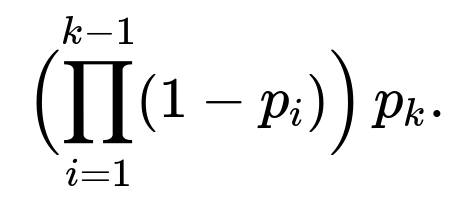
If each ( X_k ) is still i.i.d. N(0,1) but ( T_k ) changes, the probability of success changes each day. The waiting time until the first success is no longer strictly geometric, because p changes over time. Instead:
• The probability that the first success occurs on day k is


Potential Pitfalls • You cannot just take an “average p” (unless the threshold changes in a very mild or random manner). You need to be careful about exactly how ( T_k ) evolves. • If ( T_k ) eventually becomes so low that success is guaranteed, you could get a trivial finite expected waiting time, or if ( T_k ) becomes extremely high, you might never succeed.
Real-World Subtleties • This scenario appears in settings where “alarm thresholds” might adapt over time based on external conditions. • If the threshold is dynamic, you might want a day-by-day approach or a Monte Carlo simulation to estimate how quickly you will see a success.
How do you construct a confidence interval for the expected waiting time in practice?
When we say the expected waiting time is around 44 days, that is a point estimate. In practice, we might want a confidence interval around it. For a geometric distribution with parameter p, the expectation is ( 1 / p ). But p is estimated from data if we do not know it exactly. That means:
We gather samples from the underlying distribution (or historical data) to estimate ( p = P(X > 2) ).
Let ( \hat{p} ) be the empirical estimate of that probability.
The expected waiting time estimate is ( \widehat{E[N]} = 1 / \hat{p} ).
To build a confidence interval, we might do:
• A basic approach: If we have n i.i.d. samples from the normal distribution and c of them exceed 2, then ( \hat{p} = c/n ). One can use, for instance, a Wilson or Clopper-Pearson confidence interval for a Bernoulli proportion. Then invert the bounds on ( p ) to get bounds on ( 1/p ). • Alternatively, one can apply the parametric knowledge that the distribution is N(0,1), though typically if we truly know X ~ N(0,1), p is fixed. In real life, we might not know the distribution or the true standard deviation.
Potential Pitfalls • Directly inverting the confidence interval for p can produce asymmetric confidence intervals for ( 1/p ). • If p is small, sampling variation is large, meaning c can be zero if n is not sufficiently large. That leads to an undefined estimate for ( 1/p ).
Real-World Subtleties • Rare event estimation is notoriously tricky. You often need many more samples to accurately pin down p. For thresholds like 3 or 4 standard deviations above the mean, the sample size needed to reliably estimate p can be prohibitively large.
What happens if we only have limited historical data to estimate ( p )?
Sometimes, you do not know the distribution is truly standard normal (N(0,1)), or you do not trust the theoretical assumption. Instead, you measure a real process for, say, 100 days of data, and you observe the fraction of days that exceed 2. If you see only 1 day in 100 that exceeds 2, you get ( \hat{p} = 0.01 ), which is less than the theoretical 0.0228.
Issues and Edge Cases • With small sample sizes, this estimate might be unreliable or have high variance. • If you see 0 days out of 100 exceed 2, you might incorrectly conclude that p=0. Then your expected waiting time is infinite by that naive approach.
Practical Approaches • Use confidence intervals for the proportion of exceedances. A standard rule of thumb for Bernoulli p is to get at least 5–10 successes for a stable estimate, which might require thousands of days for events that happen ~2% of the time. • Consider Bayesian methods with a Beta prior for p if sample size is limited. That can produce a posterior distribution for p, from which you can get a posterior distribution for the waiting time.
Real-World Subtleties • If the process changes over time (concept drift), historical data might not reflect current or future p. • The cost of waiting for additional data might be high if you need a more precise p.
How would the analysis change if X had a heavy-tailed distribution instead of a normal distribution?
A heavy-tailed distribution (e.g., Cauchy, Pareto, or some forms of stable distributions) can have a much higher probability of large outcomes compared to a normal distribution. For instance, if ( X ) is Cauchy(0,1), the tail decays more slowly than an exponential. In that case:
• The probability ( P(X > 2) ) might be larger or smaller depending on the distribution’s tail shape, but typically for heavy-tailed distributions, you do not get the same exponential decay as in the normal. • The concept of standard deviation might not even be well-defined for certain heavy-tailed distributions like Cauchy (where the variance is infinite).
Pitfalls • If you assume normal tails but the true distribution is heavier-tailed, you might drastically underestimate how often large values occur, leading to underestimates of p for large thresholds. • You cannot use normal-based tables or tail approximations.
Practical Approaches • Fit or estimate the tail of the distribution directly, possibly with extreme value theory (e.g., Generalized Pareto Distribution). • Once you have an estimate for ( p = P(X > 2) ), the waiting time formula ( 1/p ) for the first exceedance still holds, but how you get p changes drastically.
Real-World Subtleties • Financial data often have heavier tails than normal. If you are waiting for an extreme return, you must carefully calibrate your tail assumptions. • Environmental phenomena (e.g., wind gusts, earthquakes) might also exhibit heavy tails, so normal assumptions can be misleading.
Could we use a Poisson process perspective if we were sampling continuously instead of once per day?
If draws are happening continuously in time (for instance, a sensor that samples multiple times per second), you might model exceedances as a Poisson process if the events occur independently in continuous time with a certain rate (\lambda). Then:
• The expected time until the first exceedance (the waiting time in a Poisson process with rate (\lambda)) is

• (\lambda) would be related to the fraction of samples that exceed the threshold per unit time.
Edge Cases • The Poisson process assumption might fail if exceedances cluster in time (violating independence). • Translating from a discrete “draw once per day” scenario to a continuous-time sensor reading can drastically change how we conceptualize waiting time.
Real-World Subtleties • In practice, if the sensor data are high-frequency but correlated, the Poisson assumption won’t hold. You may need specialized models (e.g., Hawkes processes for self-exciting behaviors). • The concept of “days until exceedance” might be replaced by “hours/minutes/seconds until exceedance,” depending on the sampling rate.
If we care about X exceeding a dynamic threshold that depends on the sample mean or variance from prior days, how would we proceed?
Sometimes a threshold is a function of running statistics, such as “exceed the current sample mean plus 2 sample standard deviations.” In that scenario:
Each day, you gather a new draw ( X_k ).
You update your estimates of the mean and standard deviation of all draws seen so far.
The threshold for day ( k ) becomes something like

Then you check if ( X_k > T_k ). Because ( T_k ) is random and depends on prior draws, the distribution of events “( X_k > T_k )” is even more complicated. This scenario is not a simple i.i.d. Bernoulli trial from day to day; it’s an adaptive process:
• The probability of success on day k depends on all the data up to day ( k-1 ). • Analytical solutions become quite involved.
Pitfalls • The process might have time-varying or cyclical effects. If the underlying distribution is truly N(0,1), but you keep re-estimating it from small samples, your threshold might fluctuate significantly. • The waiting time distribution might be heavily impacted by how quickly the sample mean and sample variance converge.
Real-World Subtleties • In control chart methodologies (like Shewhart charts in quality control), thresholds are typically set from historical data or from theoretical knowledge of the process. If the process is truly stable and in-control, the threshold might be fixed. If it’s out-of-control, you do additional analysis. • Using dynamic thresholds is common in anomaly detection where you adapt your threshold to new data. The waiting time until an anomaly can shift drastically as the threshold changes.
How might Bayesian updating change our perspective on waiting time for an exceedance?
Suppose we do not know the distribution parameters (mean or variance) and want to adopt a Bayesian viewpoint:
We begin with a prior on the parameters of X (mean, variance, or shape if not normal).
Each day we draw an ( X_k ), update our posterior distribution on the parameters.
Then we compute the posterior predictive probability that ( X_{k+1} > 2 ).
Our estimate of the expected waiting time is no longer a simple closed-form expression:
• On day k, the success probability (exceeding 2 on day k+1) is integrated over our posterior on the parameters. • The day-by-day probability changes as our posterior changes.
Pitfalls • Implementation can be more complex: Markov Chain Monte Carlo or other Bayesian computation might be required each step. • If the probability is small, convergence to a stable posterior can be slow.
Real-World Subtleties • Bayesian methods let us incorporate prior beliefs (e.g., that the distribution is roughly normal with unknown mean/variance) and refine them with data. • The waiting time might be heavily influenced by the prior if data are sparse.
What is the distribution of the maximum value observed after ( n ) days, and how does it relate to the waiting time for an exceedance?
Another approach to see how quickly we might observe a value above 2 is to analyze the distribution of ( \max(X_1, X_2, \dots, X_n) ). For i.i.d. standard normal draws:
• The CDF of the maximum after ( n ) draws is
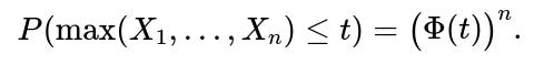
• Hence the probability that the maximum does not exceed 2 after ( n ) days is

• This is exactly the same as the probability of failing all Bernoulli trials for n days, so it’s consistent with our geometric framework.
Pitfalls • People sometimes try to use approximate extreme value distributions for the maximum (Gumbel, Frechet, etc.), but for moderate n, direct formulas or numeric evaluation might be simpler. • The distribution of the maximum is not memoryless, though the day-to-day success/failure approach is.
Real-World Subtleties • In some contexts (like stress testing), analyzing the distribution of maxima can be more natural. • If we keep running the experiment beyond day n, the distribution of the maximum changes. We must be consistent in how we handle indefinite horizon vs. finite horizon.
What if we want the probability that by day n we have at least one exceedance, but conditioned on the knowledge of partial observations?
In a real-time scenario, it might be day k, and you have not yet seen a value above 2. You might then want the probability that you see an exceedance by day n > k, conditional on the fact that you have had no exceedance so far. Under the i.i.d. assumption:
• If we have had no exceedance in k days, that means we have had k “failures” in Bernoulli terms. The memoryless property tells us that from day k+1 onward, the process “resets.” • The probability that we do not see an exceedance by day n (given no exceedance so far) is

and so the probability of at least one exceedance by day n is

Pitfalls • Forgetting the memoryless property (which only applies if draws are i.i.d.) can lead to incorrect inferences. • If the daily draws are correlated or if p changes over time, this straightforward formula doesn’t hold.
Real-World Subtleties • This is often encountered in maintenance or reliability contexts: if a system has not failed for k days, the probability of failure in the next d days might still be d * p if the system is memoryless, or it might not if the system ages. • In some domains, a “lack of failures” might update the estimated p, so the assumption that p is unchanged can be questionable.