ML Interview Q Series: Estimating Uniform Distribution Bounds using Maximum Likelihood Estimation (MLE)
Browse all the Probability Interview Questions here.
Suppose we collect n observations from a uniform distribution that spans the interval [a, b]. How can we determine the MLE estimators for a and b?
Comprehensive Explanation
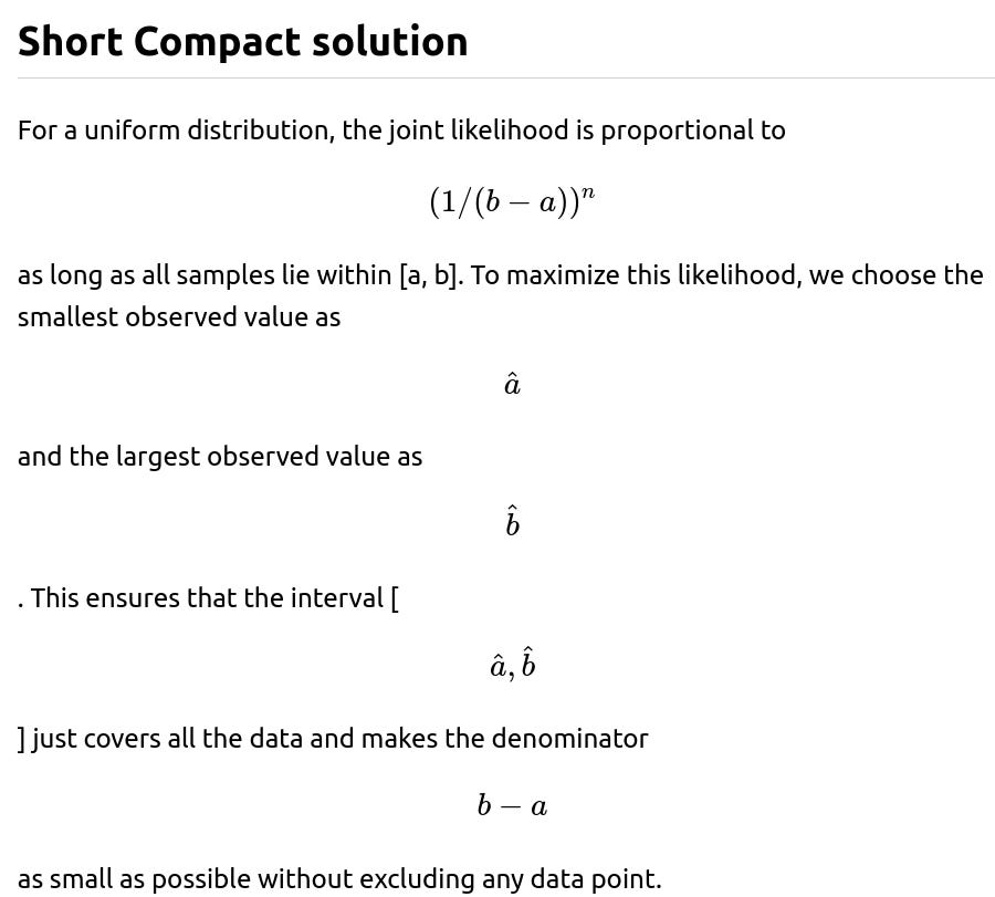
Understanding why the MLEs are the minimum and maximum of the observed samples requires us to look at how the likelihood function behaves for a uniform distribution. If we have samples


but this expression is valid only if all

lie in [a, b]. Otherwise, the likelihood is zero. Hence, we want to choose a and b so that none of the data points lie outside [a, b], while also making the length of the interval (b − a) as small as possible, because the likelihood is inversely proportional to (b − a).
From that reasoning, to keep all points within [a, b], we must have


This is the key idea behind the maximum likelihood estimation for a uniform distribution.
Practical Implementation in Python
Below is a quick code snippet (just for illustration) showing how one might compute these estimates from an array of data:
import numpy as np
def uniform_mle_estimates(samples):
"""
Return the MLE estimates for parameters a and b of a uniform distribution
given a numpy array of samples.
"""
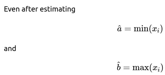
a_hat = np.min(samples)
b_hat = np.max(samples)
return a_hat, b_hat
# Example usage:
data = np.array([2.5, 3.7, 2.9, 4.1, 3.0])
a_est, b_est = uniform_mle_estimates(data)
print("MLE for a:", a_est)
print("MLE for b:", b_est)
This will output the minimum value in data as the estimate of a, and the maximum value in data as the estimate of b.
Follow-up question #1
What happens if you compute these estimators for a small sample size, and are they biased or unbiased?
It turns out that the MLE estimators for a and b in a uniform distribution are biased. For instance, consider the true parameters a and b. The MLE for b (the maximum of the sample) tends to be smaller than the true b on average if we have only a small number of observations. A similar argument holds for a. However, being biased does not always mean the MLE is a poor choice in practice; often it is still the most common estimator because it is straightforward and has desirable asymptotic properties (it is consistent as n grows large).
In fact, there are well-known bias corrections for the uniform distribution estimates. One can derive an unbiased estimator for b using a factor

multiplied by the sample maximum and similarly adjusting the sample minimum by a small fraction. This is related to the fact that the distribution of the sample maximum (or sample minimum) has a known Beta distribution relationship in the uniform case.
Follow-up question #2
Is there an alternative approach, such as a Bayesian approach, to estimate a and b for a uniform distribution?
Yes. In a Bayesian framework, you would introduce a prior over a and b and then update that prior to a posterior distribution based on the observed data. A common choice might be to assume that a and b have some diffuse prior (for example, a noninformative prior). In such a scenario, the posterior might become complicated to work with, but you can sample from it using Markov Chain Monte Carlo (MCMC) methods. Alternatively, if you have a conjugate prior (in cases of certain parameterizations), the posterior can be derived in closed form. However, for the standard parameterization of the uniform distribution, there is no simple conjugate prior, so practitioners often resort to numerical methods or choose a particular constraint or transformation of (a, b) for more tractable priors.
Follow-up question #3
How would you extend your approach to handle scenarios where you suspect outliers that might stretch the range artificially?
One strategy is to use robust estimation approaches. If you suspect outliers, your estimate of b might become very large (or a might become very small) because of a single extreme data point. Some approaches include:
Truncating or winsorizing the data to reduce the influence of outliers, then applying the MLE approach on the trimmed set.
Employing a prior that strongly penalizes extreme values of a and b in a Bayesian approach, thereby preventing a single sample from pushing the interval boundaries too far.
Using alternative distributions that model outliers explicitly, though that deviates from the assumption of a perfect uniform distribution.
In real-world practice, the uniform distribution assumption is often used as a simple first approximation or for certain bounding analyses. As soon as data exhibit outliers or other structure, more flexible models typically come into play.
Below are additional follow-up questions
Follow-up question #1: What if the underlying data does not fully come from a uniform distribution but rather a mixture of uniform and another distribution?
One must remember that the MLE approach for a uniform distribution critically depends on the assumption that every data point truly comes from a single uniform distribution across [a, b]. If the true data-generating process includes a mixture component (for example, 80% of the data from Uniform(a, b) and 20% from some other distribution), fitting a single uniform model will likely yield misleading parameter estimates.
Identifying mixture components: You might first look at descriptive statistics or visualizations (histogram, box plot, or kernel density estimate) to see if the data resemble a unimodal uniform shape. If strong deviations appear, for instance, a secondary peak, it could signal that a single uniform model is inadequate.
Handling mixture models: A straightforward approach to handle mixture distributions is to explicitly fit a mixture model. In such a scenario, you could treat the parameters (like a, b for the uniform component, and additional parameters for the other components) within a maximum likelihood or Bayesian framework, typically involving the Expectation-Maximization (EM) algorithm or MCMC for inference.
Effect on the uniform MLE: If the data contains points that belong to the other distribution with values well beyond the main cluster of uniform data,

Follow-up question #2: How do we derive confidence intervals or credible intervals for a and b under the uniform MLE framework?
, practitioners often want to quantify the uncertainty around these estimates.
Parametric bootstrapping: One approach is to use bootstrapping. You would resample (with replacement) from the observed dataset repeatedly to create many pseudo-datasets. For each pseudo-dataset, recompute the MLE for a and b. Then use the variability across these bootstrap estimates to form empirical confidence intervals.
Analytical approach: In some cases, you can use the known distributional properties of the sample extrema. For example, the distribution of the sample maximum of n observations from Uniform(a, b) is Beta(n,1)
-related when scaled to [0, 1]. Leveraging that, you can derive intervals with guaranteed coverage. However, the details can become tricky, especially if you must do a joint interval for both a and b simultaneously.
Bayesian credible intervals: From a Bayesian perspective, you would place a prior on a and b, compute (or approximate) the posterior distribution, and then derive intervals that contain a certain posterior mass (e.g., a 95% credible interval). Although there is no conjugate prior for the standard parameterization, one can specify hierarchical or transformation-based priors and sample via MCMC.
Follow-up question #3: How do we handle interval-censored data or incomplete observations when estimating a uniform distribution?
In certain real-world situations, we do not directly observe the full dataset; some observations might only be known within intervals (censoring) or might be missing entirely.
Interval-censored data: Suppose each observation is only known to lie in [L_i, U_i], instead of a precise value x_i. If any of these intervals is entirely outside [a, b], the likelihood becomes zero. Otherwise, you must consider the likelihood contribution from all feasible x_i in [L_i, U_i]. For uniform distributions, each feasible x_i is equally likely, so the data constraints effectively say that [a, b] must cover all [L_i, U_i]. The MLE will still push a toward the minimum of all L_i and b toward the maximum of all U_i.
Likelihood-based approaches: In advanced scenarios, you would form the full likelihood that accounts for the partial information. Maximizing that likelihood might be more involved than simply taking minima or maxima, especially if there are additional constraints or multiple types of censoring.
Practical difficulties: If the intervals [L_i, U_i] are quite large, the parameter uncertainty grows significantly. You may need large sample sizes or more precise interval information to get tight estimates of a and b.
Follow-up question #4: How does the estimation change if we only observe data known to be strictly bounded within [0, 1], but we do not know the exact sub-interval?
Imagine we know each sample x_i is in [0, 1], but suspect the actual distribution is uniform over [a, b], where 0 ≤ a < b ≤ 1, but a and b are unknown.
Constrained MLE: Here, you must ensure that a ≥ 0 and b ≤ 1. The MLE then is:

Because we know the distribution cannot extend outside [0, 1], we clamp the MLE to that range. If the sample minimum is negative (which is impossible if we trust the domain knowledge), it would be set to 0. Similarly, if the sample maximum is above 1, it would be set to 1. In practice, your data might never violate those bounds if the domain knowledge is accurate.
Practical interpretation: This kind of bounding can happen in applications where the quantity measured logically cannot exceed certain limits (e.g., proportions, probabilities, or pH levels in some contexts if restricted). The MLE approach remains the same, but the final estimates are pinned to the feasible region [0,1].
Follow-up question #5: What if we only need to estimate the midpoint (i.e., (a+b)/2) and the length of the interval (i.e., b-a)? Does that change the approach?
Sometimes you only care about the center or the width of the uniform interval rather than the exact endpoints.

Interpretation: These are still derived from the sample minimum and maximum. There is no separate MLE procedure that independently estimates m and ℓ for a uniform distribution, because the MLE for a and b is the pair that minimizes (b - a) subject to covering the data.
Bias: Similar considerations about bias in estimating b or a will carry over when focusing on m and ℓ. With small samples, the sample range tends to underestimate the true range on average, and thus the midpoint might not reflect the true midpoint accurately. Still, for large n, the estimates become consistent.
Confidence intervals: If you want confidence intervals for m and ℓ, you could apply the same parametric bootstrap or distributional properties of the sample minimum/maximum to get intervals for these transformations.
Follow-up question #6: How do we extend MLE for a uniform distribution to multiple dimensions?

and believe it’s uniformly distributed in some hyper-rectangle. For instance, in 2D, we assume data is uniform over [a_1, b_1] × [a_2, b_2]. We then need to estimate the corners of this rectangle.
Generalization: In d dimensions, the uniform region can be defined by coordinate-wise bounds. The MLE for each dimension is again determined by the minimum and maximum of that dimension’s data. Precisely,

where x_{i,j} is the j-th coordinate of the i-th observation.
Pitfalls: As the dimension grows, the volume of the hyper-rectangle can become quite large if there are even a handful of points that lie far apart in each dimension. The sample size required to reliably estimate these hyper-rectangular boundaries also grows exponentially. In practice, ensuring that the data is truly uniform in such a multi-dimensional region is rare unless we have domain knowledge (e.g., sensor bounds in a manufacturing process).
Possible data constraints: Similar to the 1D case, we might have partial constraints on each dimension that must be respected. The MLE solution in each dimension is bounded accordingly.
Interpretation: Visualization and domain expertise become important to confirm the reasonableness of a uniform model in multiple dimensions because data can easily exhibit correlations or clustering that violate the uniform assumption.
Follow-up question #7: How can numerical stability issues arise when we compute (b - a) in extreme cases, and how do we mitigate them?
In practical implementations, one might encounter scenarios where the minimum and maximum are extremely close in floating-point representation or extremely far apart:
Precision loss: If the data points are very large in magnitude but have small differences (e.g., numbers around 10^9 with differences of less than 1), subtracting the two can lead to floating-point precision issues in (b - a). This can affect the computation of the likelihood, or any transformations based on it.
Mitigation strategies:
Use higher-precision data types, such as double precision in standard libraries, or arbitrary precision libraries if absolutely needed.
Scale or shift the data before applying the MLE. For example, if the data is known to vary within a narrow range around a large baseline, subtract out that baseline to center the data near zero.
Check for degenerate cases where min(x_i) ≈ max(x_i). In some data scenarios (e.g., sensor data that is effectively constant), the uniform distribution might become a near-degenerate case. You might have to add a tiny buffer around the min and max to avoid division by zero.
Real-world checks: Always validate that (b - a) is not extremely small or zero. If it is, that either suggests an unusual data scenario or a potential bug in data handling.
Follow-up question #8: When might the method of moments approach for a uniform distribution be more convenient, and how does it compare to the MLE?
Method of moments: The first two moments (mean and variance) can be used to solve for a and b. If X is uniform on [a, b], its mean is

Comparison:
MLE uses the min and max, while method of moments relies on mean and variance.
The MLE can be wildly sensitive to outliers (a single large observation can inflate

). The method of moments might be less sensitive to an extreme max if that outlier does not strongly affect the variance.
If the sample size is small and the data are truly uniform, MLE is typically simpler to interpret (the actual support is pinned by the sample min and max). The method of moments might place the interval too large or too small if the mean or variance is heavily affected by sampling variation.
Both approaches assume the data is uniform in the first place. If the data is not uniform, both will be inaccurate but in different ways.
Practical usage: The MLE is generally standard for uniform distributions because it directly matches the known support, while method of moments is rarely used except in theoretical exercises. Nonetheless, it’s an alternative that can be relevant, especially if you need an internal interval that stabilizes from mean and variance or if the minimum and maximum are uncertain due to measurement issues.
Follow-up question #9: Are there scenarios where maximum likelihood may fail or produce non-unique solutions?
Identical values: If all observations x_i are exactly the same (which can happen in certain contrived or degenerate cases), then the set of possible solutions for a and b includes any interval that contains that single value. Technically, the likelihood is maximized by making a and b collapse to the same point, but that is degenerate (division by zero in the density). Practically, you might interpret this as minimal numerical variation in the dataset, so the best you can do is say a ≈ b ≈ that common value or add a small buffer for numerical stability.
No feasible solution: If the data is contradictory in some way (e.g., a must be greater than the smallest data point due to external constraints, but that conflicts with the actual observed minimum), the likelihood is zero for all possible intervals, meaning no MLE solution exists.
Multidimensional corners: In higher dimensions, as discussed, the MLE approach is straightforward in principle (use coordinate-wise min and max). However, if data is partially missing or if constraints are placed on the shape of the region, you might end up with multiple equally likely solutions (especially if the bounds are not independent across dimensions). You would then rely on additional constraints or domain knowledge to select among them.