ML Interview Q Series: Evaluating Search Algorithm Performance Using Ranking Metrics and A/B Testing

📚 Browse the full ML Interview series here.

30. How would you compare the results of two different search algorithms? How do you incorporate the rankings of the results?

One way to compare the results of two different search algorithms is to look at how effectively each algorithm places the most relevant documents at the top of the returned list. This involves understanding how we measure the relevance of each result and how we measure the overall ranking performance of the algorithm. The general process often starts by constructing a labeled dataset of queries with judgments on which documents are relevant (and perhaps how relevant). Once these judgments are in place, we can apply a variety of ranking-focused metrics to each search algorithm’s output.

There are offline evaluation strategies that focus on analyzing a set of queries with known relevance labels. Common metrics include Mean Average Precision, Normalized Discounted Cumulative Gain, Mean Reciprocal Rank, Precision at k, and others that capture how well the top-ranked documents match the ground-truth relevance information. These metrics are specifically designed to account for the order in which documents appear. For example, Normalized Discounted Cumulative Gain discounts relevant documents when they appear lower in the list, reinforcing the importance of highly relevant documents in the top positions. Meanwhile, rank correlation measures like Spearman’s rank correlation coefficient or Kendall’s Tau can compare two ranked lists directly, although these metrics tend to be more commonly used to see how two rank orderings relate, rather than focusing on absolute relevance.

In real-world systems, online evaluation through A/B testing is also important. Even if an offline metric suggests one algorithm is better at ranking, real user behavior might indicate otherwise. In online tests, user engagement metrics like click-through rate, dwell time, or user retention can provide further evidence of how effective a search algorithm is. If the changes are subtle, a statistical significance test (like a t-test or non-parametric tests) helps ensure that any difference in metrics is not simply due to chance.

When incorporating rankings of the results, it is crucial to use metrics that explicitly account for position. Algorithms that present relevant items too far down in the ranked list can negatively impact overall user satisfaction. Hence, search researchers prefer metrics like Discounted Cumulative Gain and its normalized variant (NDCG) because they apply a weighting factor that depends on position, penalizing relevant documents placed at lower ranks. Average Precision, on the other hand, integrates the notion of precision at each relevant document’s position and then averages across all relevant documents.

One must be mindful of how to handle ties, incomplete judgments, or queries that have multiple acceptable answers with varying degrees of relevance. Furthermore, in production settings where new documents appear continuously, there must be processes to update or validate the relevance ground-truth so that the evaluation remains current. Proper confidence intervals or significance testing must be carried out to confirm that observed differences between two search algorithms are meaningful and not just random fluctuations in user behavior or dataset composition.

Offline Evaluation with Ranking Metrics

It is common to create a set of queries and gather ground-truth relevance judgments for each query-document pair. A typical pipeline would involve computing multiple metrics:

Mean Average Precision (MAP) computes the average of the precision values for every relevant document retrieved, and then takes the mean of those averages across queries. This metric reflects the position of each relevant item.

Mean Reciprocal Rank (MRR) focuses on the position of the first relevant document and is suitable when there is typically a single highly relevant answer (for example, question-answer retrieval).

Precision at k (P@k) is concerned with how many of the top k results are relevant. It captures near-top quality but does not consider positions beyond k or the ordering within that top k set.

Recall at k (R@k) highlights how many relevant documents are retrieved in the top k. This is sometimes used in conjunction with precision to get a sense of overall coverage.

Normalized Discounted Cumulative Gain (NDCG) incorporates the position of the relevant documents in a way that heavily rewards relevant documents appearing earlier in the list. It also allows varying degrees of relevance (e.g., highly relevant, moderately relevant, etc.). This is one of the most popular metrics for ranking problems because it provides a smooth penalty for placing relevant documents lower in the list.

When comparing search algorithms A and B, one might compute these metrics on the same test set and then compare mean results. For instance, if NDCG@10 is significantly higher for algorithm A than for B, it means that at the first ten positions, A systematically surfaces higher-quality documents. If the improvement is large enough and statistically significant, it indicates that A is likely the superior approach for that dataset.

There may be times, however, when you want to see if the two rankings differ in a systematic way. In such cases, rank correlation coefficients like Spearman’s or Kendall’s Tau provide a measure of how the entire ordering differs. These coefficients compare the pairwise ordering of items in the two rankings. If they are highly correlated, it suggests that the difference between the two algorithms might be minor. If they are uncorrelated, it implies the algorithms produce fundamentally different orderings.

It is frequently helpful to visualize the difference in rankings to spot patterns, such as whether one algorithm is consistently good at placing certain categories of documents at the top while the other is not.

Online Evaluation and A/B Testing

Another perspective is gained by measuring how users respond to each algorithm’s results in a live setting. In an A/B experiment, a portion of the user base is routed to algorithm A, and another portion to algorithm B, over a period of time. User engagement metrics (click-through rates, session success rates, dwell time, or the likelihood of subsequent refinements) can be recorded. If users consistently interact more positively with results from algorithm A, it can indicate that A is better aligned with real-world search needs, even if offline metrics suggest otherwise.

It is also important to run significance tests (like Student’s t-test or non-parametric alternatives) on your chosen metrics to confirm that any differences observed are unlikely to be due to random chance. Because large-scale websites generate massive amounts of data, even small differences can be statistically significant, so you must consider practical significance as well.

Practical Considerations and Pitfalls

Comparing two search algorithms can be complicated by issues like incomplete judgments. Real-world labeled datasets rarely capture all possible relevant documents. This can skew offline metrics if an algorithm surfaces documents not previously considered during the labeling process. Periodic re-labelling or dynamic judgments can help keep the evaluation set more accurate.

Handling ties is another subtlety. Sometimes multiple documents have the same estimated relevance. Some metrics require tie-breaking rules or may ignore ties. In correlation-based metrics, ties can make the correlation coefficient slightly less intuitive, so it is important to define how you count or break ties if they arise often.

Particular user populations may react differently from the average user base. If you have a large global audience, you might find that while algorithm A performs better overall, algorithm B could be superior in certain regions or language groups. This kind of segmentation analysis is often done post hoc to ensure that improvements are robust across user segments.

Illustration of How to Compute NDCG

There is a commonly used formula for Discounted Cumulative Gain (DCG). The formula for DCG at position k might be expressed as follows, where

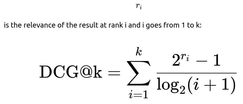
This formula sums over a discount term that grows with the rank i, thereby penalizing relevant items that appear further down the list. NDCG then normalizes this value by the best possible DCG, often called IDCG (Ideal DCG), which is computed by placing the most relevant documents at the top.

An example Python snippet for computing NDCG@k:

import math

def dcg_at_k(relevances, k):
    dcg_val = 0.0
    for i, rel in enumerate(relevances[:k], start=1):
        dcg_val += (2**rel - 1) / math.log2(i + 1)
    return dcg_val

def ndcg_at_k(relevances, k):
    actual_dcg = dcg_at_k(relevances, k)
    sorted_relevances = sorted(relevances, reverse=True)
    ideal_dcg = dcg_at_k(sorted_relevances, k)
    if ideal_dcg == 0:
        return 0.0
    return actual_dcg / ideal_dcg

In this snippet, the list “relevances” might look like [3, 2, 0, 1, 2], indicating that the first document is highly relevant (3), the second is moderately relevant (2), etc. By comparing ndcg_at_k for two separate algorithms, you gain insight into which algorithm places higher relevance nearer the top of the ranked list.

Comparing Algorithms in Practice

In practice, the comparison process involves picking one or more of these metrics, applying them to both algorithms, and then running significance tests. If algorithm A has a higher average NDCG@10 across many queries and the difference is significant, that is often enough evidence to conclude that A is an improvement. If it is not feasible to get reliable labels for every query, then an online user study or a large-scale A/B test can help confirm which algorithm better meets real user needs.

One additional subtlety is that user interface changes sometimes overshadow or confound the differences in algorithms. An algorithm that is slightly worse in terms of offline metrics could appear better to the user if it is integrated with a simpler or more intuitive interface. Hence, in real-world conditions, you would try to isolate the effect of changes in the ranking logic from other product changes.

It is also worth noting that if you are dealing with new forms of result sets (e.g., a mixture of text, images, or video), your relevance definitions and labeling standards must be carefully considered. The complexity of “relevance” grows when you consider multiple media types or multiple dimensions of a result’s utility. This complexity underscores the need to carefully define what “better” means in the context of your specific search application.

What if you have incomplete or partial relevance judgments in your dataset?

When your dataset contains incomplete or partial judgments, you face the challenge that some truly relevant documents might remain unlabeled. This can affect the reliability of offline metrics. One strategy is to collect relevance judgments only for the top k documents returned by each algorithm of interest. This forms a pool of documents likely to be relevant. You can then label those pooled results more comprehensively, thereby increasing coverage for the set of documents that matter most in the rankings.

Another mitigation approach is to adopt metrics robust to incomplete judgments. Some research suggests that metrics like bpref, which counts how many nonrelevant documents are ranked above relevant documents, can be less sensitive to missing relevance judgments. Even so, if you only have partial judgments for certain queries, your evaluation might systematically bias one algorithm over another if that algorithm tends to rank previously unseen documents that lack labels. A pragmatic approach often involves regularly updating your labeled set, focusing on the documents that appear in the top ranks of either algorithm.

Confidence intervals can be produced for your metrics through resampling or bootstrapping, so that you can better quantify how uncertain your evaluation might be due to incomplete labeling. If these intervals are large and overlapping between algorithms, you might be unable to confidently make a distinction between them until you obtain more relevance judgments.

When would you prefer rank correlation metrics like Kendall’s Tau or Spearman’s over conventional relevance-based metrics?

Rank correlation metrics measure how similarly two lists are ordered. They are useful when you want to quantify the level of agreement between two ranking functions. For instance, suppose you already have a reference ranking produced by a baseline algorithm or by human experts in a purely ordinal sense. In that scenario, you might want to see if the new algorithm’s ordering is similar or different without explicitly quantifying the difference via a relevance-based metric. If your task does not have finely grained relevance labels but only a forced ordering, then correlation-based metrics might be more suitable.

Conventional metrics like NDCG or MAP require explicit relevance judgments, potentially with multiple levels of relevance. If your data consists only of a single sorted list of items, or you are primarily interested in whether two algorithms produce the same ordering, a direct rank correlation measure is simpler and more transparent. However, rank correlation measures do not directly incorporate user-centric importance of being placed at the top. As a result, they might fail to highlight performance differences where one algorithm better promotes the most relevant documents to the top, because correlation metrics treat all positions in the list somewhat uniformly in terms of pairwise agreement or disagreement.

In many production search engines, the main concern is the actual usefulness of the top results. If that is your priority, measures like NDCG or MAP might give a more faithful representation of user-perceived quality.

How does statistical significance testing factor into comparing two search algorithms?

Statistical significance testing ensures that any observed difference in your chosen metrics, such as average NDCG or click-through rate, is not simply a random fluctuation. When you collect enough queries in an offline setting or enough user sessions in an online A/B test, you can compute the mean value of your chosen metric for algorithm A and B, then measure the variance around those means.

In an offline setting, you might treat each query as one sample of your metric and compute a t-test or Wilcoxon signed-rank test comparing the per-query metric values of the two algorithms. If the resulting p-value is below your chosen threshold (e.g., 0.05), you can be reasonably confident that your difference is not random. However, significance does not necessarily mean practical importance. A difference can be statistically significant but small in magnitude, so you should also examine effect sizes.

In online experiments, each user session or user query may be considered a sample. A standard approach is to run an A/B experiment for a defined period until you gather enough user interactions to reliably estimate the average metric for each algorithm. Then you apply the appropriate hypothesis test to see if the difference is significant. If you have extremely large traffic, almost any difference could become statistically significant. That’s where you might look at practical significance or business metrics like user engagement improvements, revenue, or user retention.

One important detail is that in A/B testing, each user might generate multiple queries or sessions, and these sessions might be correlated. Proper statistical testing can account for correlation and repeated measures. Sometimes robust or non-parametric tests are used if the data is skewed or not normally distributed.

Could you give an example of how you might structure an A/B test for evaluating two search algorithms?

A typical approach is to randomly split incoming queries or sessions into two buckets. Suppose you have 10% of traffic flow into the experimental (Algorithm B) bucket and 10% of traffic flow into the control (Algorithm A) bucket, while the remaining 80% might continue to see the existing production system or simply be unexposed to the experiment. By randomizing at the user or session level, you can mitigate systematic differences.

You then measure engagement metrics. One straightforward metric is click-through rate on the top result, or you might measure how many clicks users make before they give up. Another metric might be dwell time: how long a user stays on a clicked result before returning to the search page. Over the course of a week (or any time frame sufficient to accumulate robust data), you compare the aggregated metrics from the experimental and control groups. If dwell time is consistently higher for the new algorithm, you might interpret that as an improvement. You would then apply significance testing to see if the difference is statistically meaningful.

It is often advisable to keep the user interface identical across both conditions if you truly want to measure the difference caused by the ranking algorithm alone. If you must simultaneously test an interface change, you could run a separate experiment or isolate that variable in a multi-factor experimental design. Either way, the logic is to gather a large enough sample size so that natural day-to-day fluctuation in user behavior or traffic patterns does not overshadow the difference caused by the new algorithm. Stopping an A/B test too early may lead to false positives or false negatives due to high variance in user behavior over short time windows.

What if the new search algorithm shows better offline metrics but worse online metrics?

In practice, there can be a discrepancy between offline metrics and online user behavior. Offline metrics are only as good as your ground-truth judgments, which can become stale or might not capture the full spectrum of relevance for real users. Users also have behaviors or preferences that are not reflected in your offline dataset. For example, one algorithm might produce results that match “formal” relevance standards well, but the other might show results that are more topical or interesting, leading to higher user engagement.

When there is a conflict, the online A/B test result generally takes priority because it represents real user interaction. If you trust the methodology of your A/B test, you often accept that your offline metrics may be missing some aspect of relevance or user preference. One resolution is to revise the offline relevance assessment process, possibly by incorporating more diverse judges or more context-dependent labeling instructions. Another resolution is to add user-centric features or signals to the offline training and evaluation procedure. It is also worth doing more in-depth diagnostic analyses, for example by examining the queries or user segments for which the new algorithm does worse.

How can you deal with queries that have many equally relevant results?

There are scenarios (for example, a broad query like “cute puppies” or “landscape photography”) where multiple search results are comparably relevant. In a scenario with many equally relevant items, metrics like MAP or NDCG will not always discriminate strongly between algorithms if both produce sets of relevant items. If all relevant documents truly have identical utility, then a user might not care which relevant document is first. However, in real life, even for queries with many “relevant” documents, the user might have some preference for novelty, diversity, recency, or a certain style or format. Incorporating these additional signals can help you differentiate between algorithms.

If you truly have many results that are exactly equally relevant, rank correlation metrics might also be tricky because you will see more ties, which can reduce the maximum possible correlation. Some systems artificially introduce tie-breaking rules, or define sub-levels of relevance (like relevance plus factors for recency or popularity) so the evaluation can remain discriminative. Another approach is to track user behavior: if many items are equally relevant, the user might just click on the first one or two. An online metric like the fraction of queries that result in any successful click could be more meaningful in that context.

How do you incorporate user feedback or click data into evaluating different search algorithms?

User feedback signals, including clicks, dwell time, and bounce rates, can complement relevance judgments, especially when you lack a comprehensive labeled dataset. Implicit signals from users can indicate that a certain document was interesting or relevant enough to click on. This is typically done in an online setting:

You can collect interactions for algorithm A and B over a certain period, aggregating user feedback data. You then compute user-centric metrics such as overall click-through rate, fraction of users who refine or abandon the search, time to the first click, or dwell time on clicked pages.

You must carefully interpret click data because it can be noisy. Users sometimes click the first result regardless of its relevance. Position bias is a known phenomenon: items in the top slots receive more clicks simply because they are more visible. A carefully designed experiment tries to mitigate these biases, for example by randomly interleaving results from both algorithms for the same query and analyzing which results get clicked more when placed in the same positions.

Another subtlety is that you do not necessarily know if a click equals a relevant document. Sometimes, a user might click on a poor-quality document just to see if it is relevant, only to quickly return to the search page. That is why dwell time or other signals such as the user not returning to the search page are often interpreted as positive signals. Logging how frequently users are satisfied with top results or whether they reformulate the query can be more illuminating than simple click counts.

Many modern search systems also incorporate a mechanism to track longer-term engagement. If users never come back after seeing your top results, that might indicate a poor experience or, conversely, it might indicate they found exactly what they wanted. Proper definition of success or satisfaction is critical to interpreting user feedback metrics correctly.

How do you handle continuous deployment of improved search algorithms in a real system?

In a real production system, search quality is iteratively improved. New signals, new ranking models, or updated relevance judgments can arrive at any time. One common pattern is to adopt a continuous integration and continuous deployment pipeline. When new versions of the search ranking logic are developed, they are first tested against an offline dataset to ensure no regressions occur. Then a small-scale online A/B test is launched for a subset of real traffic. If the results meet certain thresholds (improvement in online metrics, no significant user experience issues), the new version is gradually rolled out to a larger fraction of traffic.

Each iteration incorporates data from the last iteration’s user studies, newly collected relevance judgments, or fresh user logs. One also accounts for changes in the document corpus (new items being added, old items being removed, content changes, etc.). This cyclical process helps ensure that the search system remains aligned with real-world needs, even as the underlying data and user expectations evolve.

Stopping rules are often built into this pipeline, specifying the minimum runtime for an A/B test and the minimum effect size to consider an improvement. Monitoring for anomalies is also essential because there might be external factors (system outages, seasonal events, or data ingestion failures) that skew the results if not properly accounted for. Automated alerts can pause or roll back a deployment if negative metrics are detected.

---

Below are additional follow-up questions

How do you handle query-based personalization when comparing two search algorithms?

One significant complication arises when one or both of the algorithms you are evaluating incorporate personalization signals (for instance, prior user behavior, location, or demographic data). If you compare two search algorithms without carefully segmenting by personalization attributes, you risk drawing incorrect conclusions because some users might see results tailored by algorithm A that differ dramatically from those produced by algorithm B for similar queries.

A common approach is to fix or control personalization signals so each algorithm is tested on the same user profile data. If you have user-level features (like past clicks or purchase history), you can randomly partition users (or sessions) into two buckets and ensure the personalization pipeline is consistent within each experiment bucket. This way, both algorithms have access to the same distribution of personalization signals.

Another pitfall is that personalizing the first query might create a “drifting” search session. If you measure metrics over entire sessions, subsequent queries in the session might reflect previous user interactions. You must decide how to manage the fact that these subsequent queries are no longer strictly independent. One strategy is to measure performance on the first query in each session to reduce confounding from prior queries, or explicitly track multi-query sessions and evaluate the effectiveness of personalization across the entire session flow.

When dealing with personalization, online metrics (like user engagement or click rates) often become more significant than offline judgments, because the notion of “relevance” is influenced by user-specific context. If one algorithm leverages personalization more effectively (e.g., highlighting known user interests), it could outperform the other in online experiments, even if their offline metrics are similar. This discrepancy underscores the importance of having an online evaluation plan that measures genuine user satisfaction.

Potential pitfalls and edge cases include:

• Incomplete user histories for new or anonymous users can lead to under-personalized (or generic) results, especially if your personalization approach relies heavily on established user profiles.

• Privacy regulations may limit the personalization signals you can use, impacting how you implement or compare personalized search algorithms.

• Over-personalization can cause filter bubbles, limiting user exposure to diverse content. You might inadvertently favor an algorithm that shows more of what users previously clicked on, instead of offering novel information.

Balancing personalization with overall relevance and fairness ensures that you draw correct inferences about which algorithm truly serves your users better.

How do you factor in zero-result or near-zero-result queries when comparing search algorithms?

Zero-result queries occur when a user’s query does not match any documents or when matches are so sparse or irrelevant that the engine displays no results. In practice, this scenario can happen with highly specific queries, misspellings, or extremely rare search terms. Near-zero-result queries might display only a few tangentially relevant documents.

When comparing two search algorithms, you must decide how to handle cases where one algorithm returns zero results and the other returns something. Do you consider the queries discarded, or do you penalize the zero-result algorithm? Often, these queries represent real user needs, so ignoring them can bias your evaluation.

One approach is to include them in your offline metrics if you can label whether a relevant document truly exists in your corpus. If a relevant document does exist but algorithm A returns zero results while algorithm B finds it, that is a straightforward performance difference that typically lowers A’s metrics. If it is a genuinely impossible query, you can label it as having no relevant documents and measure whether the algorithms can handle the scenario gracefully—perhaps algorithm A still tries to provide partial suggestions or spelling corrections, while B just fails silently.

In online evaluations, watch for user behavior signals like query reformulations or immediate site exits that might correlate with zero-result pages. If algorithm B consistently leads to fewer zero-result pages (and higher user satisfaction metrics), that is a strong indication B is more robust for the tail of queries. An important nuance is that zero-result queries might be very rare overall, so you must gather enough data to make statistically sound statements. If they represent 1% of your traffic, you need a large total volume of queries to meaningfully compare the zero-result rate between two algorithms.

Potential pitfalls include:

• Treating zero-result queries as outliers and removing them from your test set may artificially inflate both algorithms’ performance measures.

• Spelling corrections or query expansions can transform zero-result queries into queries that yield matches, so you must ensure that both algorithms have comparable improvements or submodules for query rewriting.

• Some domains (like e-commerce with a specialized product catalog) might yield frequent zero-result queries for out-of-stock or extremely specific item requests, so ignoring them would severely skew real-world performance measurement.

What if the search algorithm changes its indexing strategy or the underlying data changes rapidly over time?

When an algorithm includes an updated indexing strategy—like a different approach to term weighting, new embeddings, or changed partitioning of the corpus—this can drastically alter the set of candidate documents retrieved before ranking. The data layer (the indexed corpus) is effectively part of the search algorithm’s pipeline, so changes in how data is stored or accessed can confound direct comparisons.

To handle this, ensure that both algorithms are tested against the same snapshot of the corpus, or run them concurrently on the same, continuously updated data. If the data changes during the experiment (common in real-time or dynamic indexes), adopt a time-slice evaluation approach: fix a snapshot from day N for offline experiments or run an A/B test in real-time for the same time window for both algorithms. That way, the difference in results can be attributed to the algorithm rather than to an unshared data environment.

Rapidly changing data complicates the notion of “ground truth” relevance. A document that was relevant last week might be obsolete this week. For example, news or trending topics can shift quickly, and an algorithm that updates indexes more frequently might appear better. Indeed, the ability to handle fresh data is often a legitimate advantage. Nonetheless, you must carefully measure how each algorithm deals with stale vs. new content so you can fairly assess their relative performance.

Potential pitfalls include:

• If you freeze the corpus in an offline setting, you lose the advantage that real-time indexing confers in practice. This might understate the performance of an algorithm designed for real-time updates.

• If you run an online A/B test but algorithm A is deployed on older index servers while B is on newer ones, the difference in user satisfaction might stem from data freshness rather than ranking strategy.

• Data drift can make your offline judgments inaccurate. If your labeled set is from months ago, it might not reflect the currently indexed content. Continual re-labelling is essential for rapidly changing domains (e.g., social media, e-commerce).

Finding the right balance between controlled snapshots for offline comparison and real-time continuous data for online evaluation is key to drawing valid conclusions about which algorithm truly handles evolving data better.

How do you measure the diversity or coverage of search results in addition to relevance?

Traditional metrics like NDCG or MAP focus primarily on relevance, assuming each result’s relevance is independent of the others. However, in certain domains—like news aggregators, product searches, or exploratory search scenarios—users may benefit from a diverse set of results covering different subtopics or categories. Simply returning ten documents that are nearly identical can be less useful.

To incorporate diversity, specialized metrics can be used. One approach is to define subtopics for each query and measure “subtopic recall”—how many distinct subtopics are covered in the top k results. Another approach is the intent-aware version of NDCG that weighs coverage of known user intents. Alternatively, one might apply metrics like α-NDCG, which penalize redundancy in retrieved documents.

This can be challenging in real-world applications because you need a robust way to identify subtopics or categories. Domain knowledge often helps. For instance, for an e-commerce site, diversity might mean returning products from multiple brands, price ranges, or styles. For general web search, it might mean covering different aspects of a multi-faceted query.

Potential pitfalls and edge cases:

• Over-diversification can lead to lower overall relevance if your system is so focused on covering subtopics that it omits the most relevant items.

• Defining “subtopics” can be subjective. For queries like “rock music,” you might have subtopics around different eras, genres, or popular bands, but no universal set of subtopics covers every user’s expectations.

• Relying on user engagement signals for diversity evaluation can be noisy, as some users might prefer to see more of the same type of item, while others prefer variety.

• In an A/B test, diversity might result in higher user engagement overall, but you may see decreased precision for hyper-specific queries. You must weigh these trade-offs based on your product goals.

In practice, a balanced approach combines classical relevance metrics (like NDCG) with at least one measure of diversity, or post-reranking steps that ensure a certain level of coverage if the user’s intent might be broad or unclear.

How do you handle real-time user feedback or immediate user actions that might re-rank the results within a single session or query?

Certain search systems dynamically adjust rankings based on user signals in real time—sometimes called “session-based re-ranking” or “interactive search.” If you compare two algorithms, but one of them performs dynamic re-ranking (e.g., pushing up documents that were partially clicked or hovered over), while the other uses a static ranking, direct comparisons can be tricky.

A typical solution is to either:

1. Disable the session-based re-ranking in both systems and compare their baseline performance.

2. Keep the session-based re-ranking in both systems if you have distinct re-ranking logic in each algorithm and measure performance in a user study or an online A/B test.

When the system re-ranks results in the same session, standard offline metrics become less meaningful because the final ranking the user sees is partly decided by interaction. You might need to log each user’s initial ranking, subsequent user actions, and the system’s adjustments. Then you compute user-centric metrics like dwell time or final click positions for the actual re-ranked list.

Potential pitfalls and edge cases:

• If you only measure the first set of results ignoring the re-ranked changes, you might underestimate the true user satisfaction from a system that adaptively improves results.

• If you measure after re-ranking, you need to ensure both systems get approximately the same opportunities to learn from user signals, or you might inadvertently favor the system that has more data or more frequent re-ranking triggers.

• Real-time user feedback can be noisy, especially if a user randomly clicks around. Distinguishing meaningful signals from random exploration can be difficult.

Interpreting results in real-time interaction scenarios typically leans heavily on well-designed online experiments and sophisticated logging of user actions. This ensures that the dynamic algorithm’s benefits are fairly captured.

What are some domain-specific pitfalls when comparing search algorithms (e-commerce vs. news vs. legal vs. other domains)?

Different domains can drastically alter what “good” search results look like. A one-size-fits-all set of metrics or user engagement signals might not capture domain-specific nuances:

• E-commerce: Users often care about price, brand, shipping time, or availability. Relevance alone (matching keywords) is not enough; you may need to incorporate ranking signals that reflect product popularity, personalized preferences, or inventory. Skipping these factors could cause large discrepancies between offline relevance metrics and actual conversion or sales metrics.

• News: Timeliness is paramount. An older article might be highly relevant to a general question but stale for breaking news queries. A search algorithm that emphasizes fresh or local news could outperform another that ranks by standard relevance. Also, coverage of diverse topics or viewpoints might be more important in the news domain, complicating the measurement of success.

• Legal: The correctness and comprehensiveness of results could be far more important than a small improvement in ranking some documents earlier. Missing a crucial precedent or case reference can have significant professional ramifications. Assessing recall might take precedence over precision, which might differ from typical web search metrics that emphasize early precision.

• Healthcare: Accuracy and trustworthiness matter profoundly, and returning harmful or misleading information can have serious consequences. Relevance labeling might require domain experts, not crowd-sourced workers. This can limit dataset size and complicate evaluations.

These domain-specific factors require customizing data collection and metric design. If you rely solely on standard “vanilla” metrics (like MAP or NDCG) without domain adaptation, you risk favoring an algorithm that is suboptimal for real user needs in that field.

Potential pitfalls:

• Overemphasis on purely text-relevance signals when domain-specific factors (e.g., time sensitivity, compliance, or expert endorsements) are crucial.

• Not capturing user intent or the typical workflow (e.g., in e-commerce, the user might click multiple products and compare prices, whereas in legal research, thoroughness often matters more than quick answers).

• Missing domain subtleties like synonyms or specialized taxonomies.

A robust comparison always tailors the ground-truth judgments, labeling processes, and user metrics to the domain’s real demands.

How do you handle queries with ambiguous user intent or multiple possible user intentions?

Ambiguous queries (e.g., “Java,” “apple,” “Mercury”) can refer to entirely different topics. A user might be looking for programming language details, the fruit, or the planet. Or a single query might have multiple equally valid interpretations (e.g., “panther” could refer to the animal or sports team, or a user might want images vs. news stories).

In many such cases, an algorithm that covers various interpretations within the top few results can be more useful. Hence, measuring how well each algorithm handles ambiguity can require specialized labeling or diversity metrics. For offline evaluation, you might define separate “intents” for the query and check how well the system addresses each. If the user intent is not known in advance, you can label all plausible interpretations as relevant. Then algorithms that surface results for multiple major interpretations earlier might score higher.

In online settings, if you have user logs, you can see which link the user clicked after an ambiguous query. If the new algorithm better anticipates the user’s probable meaning, you might observe better click-through rates or fewer query reformulations. Alternatively, if the algorithm returns multiple interpretations, the user can quickly find the correct one without re-querying.

Edge cases and pitfalls:

• Some queries might have dozens of interpretations, making it impractical to label them all in offline judgments. You may have to rely on partial coverage or user feedback to gauge success.

• Intent might shift within a session. The user types “apple” first looking for the tech company, then modifies the query to “apple nutrition” to see fruit nutrition facts. A single static label might not capture this dynamic behavior.

• Large language model-based approaches might guess the “most likely” interpretation from context, but if there is no context, it can still be a toss-up. Make sure the label set accounts for multiple correct answers rather than a single best answer.

Measuring success for ambiguous queries often requires a blend of offline diversity labeling, online user engagement, and deeper session-level analysis, because intent can evolve as the user clarifies their needs.

What are the pitfalls of analyzing only average metrics across queries, ignoring the distribution of query frequency or difficulty?

Focusing solely on average metrics like mean NDCG or mean precision can mask important behavior differences. Some queries are extremely frequent (head queries), while others occur rarely (long-tail queries). It is possible for an algorithm to perform well on infrequent long-tail queries but poorly on the frequent queries, or vice versa, skewing an “average” metric if the test set does not represent the real query distribution.

A recommended approach is to segment queries by frequency or difficulty:

• Head queries: The top 5-10% of queries might represent 80-90% of user traffic. Performance on these queries can heavily impact real-world user satisfaction.

• Long-tail queries: Each might be rare individually but collectively represent a large chunk of total traffic. Handling them effectively can differentiate one algorithm from another, especially in e-commerce or specialized domains.

• Difficult queries: Even if they are not necessarily rare, they might be ambiguous or require advanced reasoning. An algorithm that is robust on these can produce better user retention.

Similarly, weighting queries by their actual frequency in production can yield a metric that better reflects user impact. Otherwise, a test set with equal representation for all queries might overrepresent rare or easy queries. Another approach is to calculate metrics separately for different segments (e.g., top 100 queries vs. next 1,000 vs. the entire distribution) and see if one algorithm is systematically stronger in certain segments.

Potential pitfalls:

• If your offline labeled set does not mirror the real query distribution, you might conclude an algorithm is superior in your test environment but discover the opposite is true in production.

• Aggregating queries with widely varying complexity into a single metric can hide the fact that an algorithm struggles with certain classes of queries that matter to your product domain.

• In an online A/B test, if you do not track performance by query segment, you might see a moderate improvement on average, but unknowingly degrade performance for your top revenue-generating queries.

Balancing average metrics with segmented or frequency-weighted analyses helps you gain a complete picture of which algorithm truly meets user needs across the entire query space.

How do you incorporate voice-based or multi-modal queries into these evaluations?

As search interfaces expand to voice (e.g., smart speakers), image search, or multi-modal queries (voice plus an image, or text plus user gestures), the evaluation becomes more complex. Traditional offline metrics that rely on textual relevance judgments might be insufficient to capture whether the system correctly interpreted a spoken command or recognized the objects in an uploaded image.

For voice-based search, the system must handle:

• Speech recognition accuracy, which can introduce errors before you even get to the ranking logic.

• Conversational context, where a user might say “Show me pictures of that” referencing a previous voice query or a real-world object.

When comparing two voice-based or multi-modal algorithms, you may need new forms of labeled data—audio transcripts, recognized text, or object detection labels. You might also track whether the user repeated or rephrased a query if the system apparently misunderstood them. Online user satisfaction metrics might involve how often the user tries the same request again or how quickly they exit.

Potential pitfalls:

• If one algorithm consistently mishears certain phrases, you might incorrectly attribute poor relevance to the ranking stage rather than to speech recognition issues.

• For multi-modal queries (e.g., voice plus an image), you need consistent ways of labeling the combined intention. Some approaches rely on user-level input or advanced context, so offline data might be limited.

• Real-time environmental noise or device differences can cause variation in speech recognition performance, making it harder to isolate ranking performance. A controlled environment might not reflect real user conditions.

Assessing multi-modal search often involves specialized pipelines for recognition or extraction (e.g., image embedding, speech-to-text). Ensure both algorithms use the same pipeline or factor out pipeline differences carefully, so you can isolate changes specific to the search or ranking logic.

What is the role of explainability or interpretability in search algorithm comparison, and how might you measure that?

Beyond just accuracy or relevance, some domains or organizational contexts require that results be explainable—for example, showing users why certain documents appeared at the top or whether certain rules or signals influenced the ranking. Traditional ranking metrics do not measure explainability, so you may need separate tests or user studies that gauge how well users understand the returned results.

One approach is to run user surveys or experiments where you provide a short explanation or highlight the key factors behind a ranking. You then compare user trust and satisfaction levels across two search algorithms—one that offers no explanation vs. one that provides a clear rationale. Though not a purely quantitative measure like NDCG, it can be vital in high-stakes domains (healthcare, legal, financial).

Pitfalls and edge cases:

• An algorithm that is highly accurate but opaque (such as a complex ensemble of deep learning models) might perform better on standard ranking metrics but worse in user trust or compliance.

• For large language models used in search, interpretability might involve showing relevant passages or citations. If algorithm B does not surface or highlight these passages as well, it could degrade user trust despite good metrics.

• Over-simplified “explanations” can be misleading if they do not reflect the true reasons behind the model’s decisions. This might cause users to develop incorrect mental models of the system.

If interpretability is a key user or regulatory requirement, you might incorporate additional user interaction metrics, measure how often users expand “explanations,” or run satisfaction surveys. You could also measure the correctness of the explanations themselves via domain experts. These forms of evaluation go beyond standard offline metrics but can be decisive in critical applications.

How do you handle adversarial or spammy behaviors from certain queries or documents, which can skew your evaluation?

In many open search systems—especially on the web—spammers or adversarial agents try to manipulate rankings. They might stuff documents with keywords, generate automated queries, or create user click bots. This can corrupt your evaluation by inflating traffic metrics or introducing misleading signals into your labeled sets.

Typical anti-spam measures include:

• Filtering out suspicious traffic or known bots before analyzing user interactions. This can be done by checking IP addresses, user-agent strings, or velocity patterns that do not match normal human usage.

• Updating the labeling guidelines to mark spam documents as non-relevant, or explicitly track “spam” as a label.

• Using robust query sampling that tries to exclude artificially injected queries. If spammers are specifically targeting certain keywords, you can examine anomalies in the query distribution to detect them.

When comparing two algorithms, if algorithm B is more susceptible to spam manipulation, it might appear worse in user engagement metrics or offline judgments if the spam documents end up being labeled as relevant or overshadow actual relevant documents. Conversely, an algorithm with stronger spam filters might produce more stable, reliable results.

Potential pitfalls:

• Overzealous filtering can accidentally remove legitimate user behavior from your test set. That can bias your results in favor of whichever algorithm is tested on “cleaner” data.

• If you run an online experiment and spammers deliberately target the new algorithm, you might incorrectly conclude it performs poorly. Continual monitoring of suspicious patterns during A/B tests is critical.

• Spam detection or ranking resilience to adversarial documents is a separate dimension of evaluation. A purely relevance-based offline dataset might not account for spam at all, so you might need specialized “spam test sets” or real-world traffic analysis to gauge resilience.

Making sure your comparisons reflect real usage requires robust spam detection and consistent data cleaning protocols across all tested algorithms. Otherwise, adversarial queries or spam-laden documents can distort your results.

How do you ensure that your evaluation metrics do not inadvertently measure something else, leading to metric gaming or overfitting to a specific metric?

When the success of a search algorithm is reduced to a single metric, engineers may optimize that metric aggressively, sometimes ignoring broader user satisfaction. This phenomenon—“metric gaming” or “overfitting to the metric”—can result in a system that is good at passing the test but not necessarily delivering the best user experience.

A common practice is to employ multiple metrics:

• Use standard ranking metrics (e.g., NDCG, MAP) for offline checks.

• Use complementary metrics like coverage, click diversity, or dwell time in online tests.

• If your business has high-level goals such as user retention or conversion rate, track those as well.

If improvements in your chosen metric do not align with better user outcomes, reevaluate whether your metric is truly capturing user value. You can also adopt continuous user feedback loops. If you see user dissatisfaction increasing despite improvements in NDCG, that is an early warning sign of misalignment.

Another approach is to rotate or expand metrics over time:

• For a given quarter, you might emphasize NDCG but also keep an eye on diversity and dwell time.

• For the next quarter, reevaluate how well your system handles zero-result queries or ambiguous queries.

Pitfalls:

• Relying on a single offline metric might incentivize trivial changes, like artificially boosting certain queries in the labeled set.

• Over-tuning to your offline dataset might degrade performance in real traffic if the dataset is not representative.

• In an online environment, simplistic metrics (e.g., raw click-through rate) can be gamed by pushing click-bait or sensational results that are not truly relevant.

Balancing multiple metrics and continuous user feedback ensures that you do not blind yourself to deeper issues or degrade overall experience for the sake of one easily measured metric.

How do you handle potential fairness or bias issues in search results, especially if your user base is diverse?

Fairness in search can refer to ensuring that certain groups, topics, or content types are not systematically disadvantaged by the ranking. Bias can creep in through training data or relevance judgments, especially if these judgments reflect the majority perspective and overlook minority contexts.

When comparing two algorithms with respect to fairness, you might define certain fairness objectives or constraints. For example:

• Measure how often search results for queries related to a minority group are relevant or positively framed.

• Evaluate representation in top results to see if certain protected categories are underrepresented or misrepresented.

This can be done using specialized fairness metrics, user surveys, or external audits. You might run an offline test set with queries that specifically focus on sensitive issues, or track user engagement among different demographic segments in online experiments.

Pitfalls:

• Defining “fairness” in search is not straightforward. Different stakeholders might have different definitions or emphasis (e.g., demographic parity vs. individual fairness).

• Over-correcting might hamper overall relevance if you forcibly inject certain results to meet fairness quotas, so a balance is necessary.

• Labeled data for fairness testing might be limited, or ground-truth definitions might be contentious.

• If your user base is global, fairness complexities might multiply across cultural contexts and languages.

Ultimately, you might find an algorithm that seems to rank results well from a purely relevance-based perspective, but inadvertently amplifies biases. Incorporating fairness checks into your standard evaluation pipeline helps avoid harmful or discriminatory outcomes, especially in sensitive domains (like job listings, housing, or healthcare information).

How do you address the cold start problem for newly introduced documents or queries in the context of algorithm comparison?

The cold start problem arises when new documents (or new queries) have little or no historical data, making it difficult for a search algorithm to accurately rank them. If algorithm B employs advanced machine learning that relies on extensive historical click data, it may underperform for newly added items compared to algorithm A, which might rely more on textual or content-based features.

In comparing algorithms, you can create a subset of queries or documents specifically labeled as “fresh” or “recently added,” then track performance on those. Alternatively, you can run an online experiment that measures how quickly each algorithm incorporates new content into relevant results. If your product domain frequently changes (like news or user-generated content), the ability to handle new data effectively might be critical.

Pitfalls:

• If your offline dataset is mostly well-established queries and documents, neither algorithm is tested on cold start scenarios. You might incorrectly conclude that the advanced ML-based approach is always better, only to find it struggles with new items in production.

• Overreliance on popularity or behavioral signals can lead to a “rich get richer” effect, where new items never surface due to insufficient signals.

• Some systems implement specialized exploration or “boosting” for new items to gather data. This can confound direct comparisons if only one of your tested algorithms has an exploration module.

Evaluating cold start performance often involves measuring recall or speed of discovery for new items, as well as user engagement on new content. The best algorithm from an overall standpoint might still be suboptimal if it consistently fails to handle new items promptly or fairly.

How do you scale your evaluation pipeline to handle extremely large datasets or real-time streams of user queries?

Large-scale search systems can process millions or billions of queries daily. Conducting offline evaluations on massive labeled datasets or running large A/B tests can be computationally and organizationally challenging. Common strategies include:

• Sampling: Randomly sample a manageable subset of queries that still reflects the real distribution. This reduces computation while preserving statistical power if done correctly.

• Distributed computation: Use cluster computing frameworks (e.g., Spark) or specialized big data tools for metric calculations. Pre-generate partial sums or aggregates so you do not recalculate from scratch each time.

• Incremental evaluation: Update metrics periodically (hourly or daily) rather than rerunning everything from scratch. This helps in near-real-time monitoring of algorithm performance changes.

• Real-time dashboards: For online experiments, feed metrics into a real-time analytics system that updates frequently. This can alert you quickly if performance anomalies arise.

Potential pitfalls:

• Poorly designed sampling strategies might exclude long-tail queries or outlier user segments, leading to biased evaluations.

• Handling large-scale data can produce memory or compute bottlenecks, so you must carefully optimize your pipeline or risk partial or incomplete metric calculations.

• Real-time analytics might show short-term fluctuations, so you need robust significance testing over aggregated periods before making final decisions.

Proper engineering and infrastructure design—like well-managed data pipelines, reproducible offline tests, and well-structured A/B frameworks—are essential. They not only provide reliable results but also allow you to iterate quickly.

What if you are migrating from a keyword-based search system to a neural or semantic search system, and you want to ensure continuity or measure improvement effectively?

Migrating from a traditional keyword-based system to a neural search approach changes both retrieval and ranking logic. Neural search might rely on dense embeddings, while the old system uses inverted indexes and keyword matching. Comparisons can be complicated because:

• The set of candidate documents retrieved may differ.

• Some user queries that never returned results might now produce relevant matches based on semantic similarity.

A step-by-step approach could be:

1. Keep the same user interface. Under the hood, compare the new neural retrieval with the old keyword-based approach on a representative test set.

2. Identify queries where neural search can excel (e.g., paraphrased or natural language questions) and queries where it might fail (e.g., rare named entities).

3. Use offline labeled data to compute classic ranking metrics but also gather specific examples where neural search yields new relevant documents the old system missed.

4. Conduct a staged online rollout. Perhaps route a fraction of traffic to the neural system. Monitor both standard metrics (click-through, dwell time) and user complaints or helpdesk tickets to see if you degrade certain specialized queries.

Potential pitfalls:

• If your offline judgments are heavily biased toward keyword-matching relevance, the neural system might appear worse because it returns documents that were never labeled. You might need an updated labeling strategy or dynamic judgment.

• Neural search could increase recall dramatically, but might occasionally include irrelevant semantically related documents. This can confuse users accustomed to precise keyword matches.

• Latency can be higher for neural search if embeddings are large or if you do not have an efficient approximate nearest neighbor index. In a real system, slower responses might degrade user satisfaction, overshadowing relevance gains.

Ensuring continuity typically involves a transition plan where you systematically measure performance across different query classes. You might also do a fallback strategy: if the neural approach fails or times out, you revert to the keyword-based system. Over time, as performance and coverage improve, you can fully adopt the neural approach.

How do you consider system latency or computational resources in addition to result relevance when comparing two search algorithms?

While relevance is crucial, in real production systems you cannot ignore latency and computational overhead. An algorithm that produces slightly more relevant results but takes much longer to return them might not be a net improvement in a live search environment. Many users will abandon slow queries, particularly on mobile devices or with limited network connectivity.

When comparing two algorithms, measure:

• Response time distribution: The median or 90th/95th percentile latency can highlight whether algorithm B has tail-latency issues (i.e., extreme slow queries).

• Resource usage: Memory consumption, CPU or GPU usage, and cost of serving. If B consumes more resources, can your infrastructure handle the scale?

• User experience metrics: If a system is slower, do users bounce more or re-submit queries?

Sometimes, to account for both relevance and latency, you might define a composite score that includes both. Alternatively, you keep them as separate but equally important metrics: if an algorithm is 2% better in NDCG but 30% slower, you might decide that is an unacceptable trade-off. Or you might optimize for the best “pareto-optimal” point, balancing the trade-off between relevance and performance.

Potential pitfalls:

• Focusing purely on average latency can hide the fact that some queries might be extremely slow. Those outliers can degrade user perception more than you might expect from average metrics.

• If algorithm B is faster but less relevant, it might artificially improve user engagement metrics simply because people do not like waiting. However, they could also be unsatisfied with the results if the speed advantage is not enough to offset poor relevance.

• Infrastructure scaling might be non-linear if the algorithm requires specialized hardware or large-scale index builds. You must factor operational complexity into your final decision.

Realistically, you want an algorithm that meets or exceeds a certain latency threshold while improving relevance. If it fails to meet that threshold, further optimization or a hybrid approach may be needed.

What is the difference between comparing two ranking algorithms vs. comparing two entire retrieval pipelines, and how do you break that difference down?

A retrieval pipeline can include multiple stages:

1. Parsing or rewriting the user’s query (spelling correction, synonyms, expansions).

2. A retrieval step that fetches candidate documents from an index or a deep neural retrieval model.

3. A ranking step that scores and reorders those candidates.

4. Possibly a re-ranking or personalization step incorporating user context or additional signals.

When you say “comparing two search algorithms,” you could mean you are only swapping out the final ranking stage while keeping the rest of the pipeline constant. Alternatively, you might be replacing the entire pipeline from query parsing to final ranking. Clarifying the scope is critical. If you only compare ranking modules but keep retrieval the same, it may not capture improvements that come from better candidate generation. Conversely, if you replace the entire pipeline, you might see differences caused by changes in synonyms or expansions, not just the ranking logic.

A recommended approach is to isolate and measure each stage:

• Evaluate retrieval changes independently (did the new retrieval approach bring better candidates?).

• Evaluate ranking changes with the same retrieval set (did the new ranking approach reorder those candidates more effectively?).

• Evaluate combined performance in an end-to-end scenario, either offline or via an online experiment.

Pitfalls:

• If you do not control for candidate sets, you cannot tell if the difference stems from the retrieval stage or the ranking stage.

• A new pipeline might involve additional data preprocessing that invalidates direct comparisons with the old pipeline.

• Typically, user behavior in an online environment reflects the entire pipeline experience, so even a small improvement in query rewriting might overshadow ranking differences.

Breaking the pipeline into modular evaluations helps you pinpoint exactly where gains come from, ensuring each subsystem is fairly assessed before final end-to-end testing.

How do you incorporate user satisfaction surveys or explicit user feedback forms in your evaluation process, and what pitfalls might arise from that approach?

Beyond click signals and relevance judgments, some systems add a user feedback mechanism: a pop-up question like, “Were these results helpful?” or a rating scale. This can be valuable for capturing explicit user sentiments, especially if you handle specialized queries or want deeper insight into user experiences.

To incorporate surveys:

• Randomly assign a fraction of users or queries to receive a feedback form, so you do not overwhelm all users or degrade the experience.

• Compare the ratio of positive vs. negative feedback across the two algorithms. This can supplement standard usage metrics (like click-through) to ensure you capture user perception.

• Use significance tests to confirm whether differences in feedback are robust or just noise.

Pitfalls:

• Feedback fatigue: If you prompt users too often, they may ignore or hastily click something just to dismiss the popup, undermining data quality.

• Selection bias: Users who respond to surveys might not be representative of all users. They might be more engaged or more frustrated.

• Leading questions or poorly designed surveys can bias responses. For instance, if you phrase a question in a way that nudges users toward a positive answer, you will not get accurate data.

• Sample size might be small if only a subset of users opts to provide feedback. You need enough responses per condition (algorithm A vs. algorithm B) to reach meaningful conclusions.

In domains where user trust and satisfaction are paramount—health, finance, legal—explicit feedback can offer more nuance than typical click signals. Nonetheless, it should be part of a broader evaluation strategy, not the sole criterion for deciding which algorithm to deploy.