ML Interview Q Series: Expectation-Maximization: Solving Latent Variable Estimation in Gaussian Mixture Models.

📚 Browse the full ML Interview series here.

Expectation-Maximization (EM) Algorithm: What is the Expectation-Maximization (EM) algorithm and how does it work? *Describe a scenario like estimating parameters for a Gaussian Mixture Model (GMM) where we have hidden variables. Outline what happens in the E-step and M-step of EM, and why EM is useful for problems with latent (unobserved) variables.*

Overview and Core Explanation

The Expectation-Maximization (EM) algorithm is a powerful iterative procedure used to estimate parameters in probabilistic models, especially in the presence of unobserved (latent) variables. The fundamental idea behind EM is that we can improve our estimate of the model parameters by alternating between:

• Inferring the distribution of hidden variables (E-step).

• Re-estimating parameters that maximize the likelihood of the data, given these inferred distributions (M-step).

The algorithm converges to a (local) maximum of the likelihood function or (under certain formulations) the posterior if a Bayesian prior is included. EM is particularly valuable when the model involves latent variables that are difficult or impossible to observe directly, or where direct maximum likelihood estimation would be intractable without introducing these latent variables.

This discussion will be illustrated with the classic example of a Gaussian Mixture Model (GMM). GMMs assume that data comes from a mixture of several Gaussian distributions, but the specific cluster or component that generated each data point is unknown (latent). This latent cluster assignment is exactly what EM helps us to infer, while simultaneously updating the parameters of the Gaussians themselves.

Gaussian Mixture Model Scenario

In a GMM, we assume we have kk Gaussian components, each with its own mean and covariance. We also have mixture weights that indicate how likely each component is. Let:

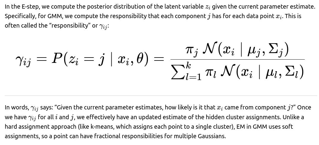
E-step (Expectation Step)

M-step (Maximization Step)

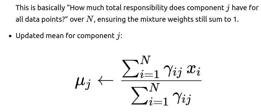
This is essentially the weighted mean of data points assigned to that component.

• Updated covariance for component j:

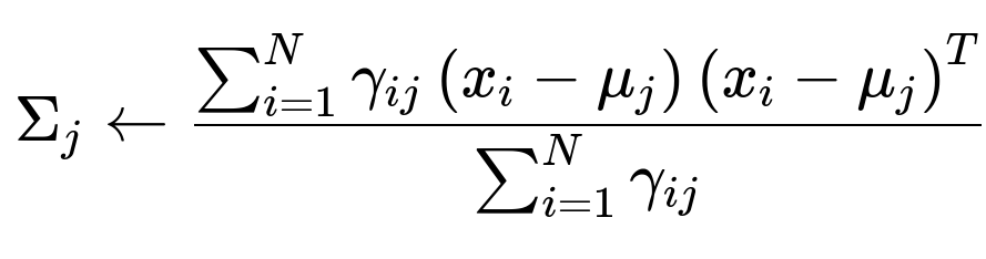
• This is the weighted covariance based on the responsibilities. (Sometimes a small regularization term is added to the diagonal to avoid singularities.)

These steps are repeated until convergence, often defined by the change in log-likelihood or change in parameter estimates dropping below a tolerance.

Why EM is Useful for Problems with Latent Variables

1. Soft Assignments: EM naturally handles partial assignments to latent categories, allowing for the possibility that any given data point might come from multiple latent components with certain probabilities.

2. Closed-Form Updates in Many Models: Many latent variable models (like GMMs, some factor analyzers, hidden Markov models) admit closed-form parameter update rules in the M-step.

3. Principled Probabilistic Approach: EM uses the complete-data log-likelihood framework, a powerful formalism that is more robust than heuristics like k-means.

4. Flexibility: EM generalizes to many kinds of mixture models and other scenarios where latent structures exist (e.g., missing data problems, clustering, dimensionality reduction, etc.).

EM can get stuck in local maxima since it is a coordinate-ascent-type procedure on a non-convex function, so initialization is often critical. Despite this, it remains a workhorse algorithm in unsupervised learning and many areas of machine learning.

Detailed Steps in GMM EM

• Initialization:

E-step:

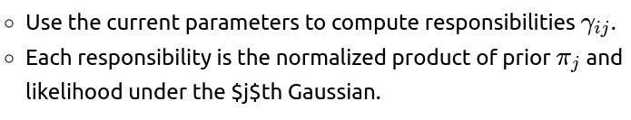
M-step:

Check Convergence:

Compute the log-likelihood of the observed data under the updated parameters:

• Compare with the previous iteration’s log-likelihood. If the improvement is smaller than a threshold or some iteration limit is reached, stop; otherwise, go back to E-step.

Below are typical follow-up questions and in-depth explanations that can arise in a FANG-level interview.

What are common convergence issues or pitfalls with the EM algorithm and how can we address them?

A major risk of EM is convergence to a local maximum rather than the global maximum, as the likelihood surface in many mixture models is non-convex. The final parameter estimates may be strongly dependent on the initialization procedure. Strategies to mitigate this include:

• Multiple Random Restarts: Run EM from different initial guesses and pick the solution with the highest final log-likelihood.

• K-means Pre-initialization: Use k-means to get initial cluster centroids, then set the mixture weights and covariances accordingly.

• Regularization: Add a small diagonal term to each covariance matrix to avoid singular matrices and to improve numerical stability.

• Monitor Log-Likelihood: Track the log-likelihood at each iteration and terminate if it stops improving or if updates begin to exhibit numerical instability.

Another pitfall occurs if a Gaussian component collapses onto a single data point, making the covariance matrix nearly singular. The regularization trick or removing/spreading responsibilities can help fix this issue.

How does the EM algorithm compare to gradient descent methods for maximum likelihood estimation?

• Gradient Descent: Typically requires computing the gradient of the log-likelihood and possibly choosing a suitable step size. It is a more general approach but can be sensitive to hyperparameters like learning rate, momentum, etc.

• EM: Rather than computing the gradient directly to perform an update, it alternates between the E-step and M-step. For models like GMMs or hidden Markov models, these updates have closed-form expressions. Hence, EM can sometimes be more direct and faster to converge in such models because each M-step is effectively a coordinate-wise optimization of a bound on the likelihood.

• Local Convergence: Both are susceptible to local maxima in non-convex likelihood landscapes. For well-structured mixture models, EM’s closed-form updates often work efficiently in practice, although it can still get stuck if initialization is poor.

Could you illustrate a short snippet in Python of how EM might be implemented for a GMM?

Below is a conceptual (simplified) Python-like pseudocode. In a production environment, you would typically use libraries such as scikit-learn or PyTorch to handle complexities and optimizations.

import numpy as np
from scipy.stats import multivariate_normal

def initialize_parameters(X, k):
    # X is shape (N, d)
    # k is number of mixture components
    N, d = X.shape
    np.random.seed(42)
    # Randomly initialize means
    means = X[np.random.choice(N, k, replace=False)]
    # Initialize covariances (as identity)
    covariances = np.array([np.eye(d) for _ in range(k)])
    # Initialize mixture weights equally
    weights = np.ones(k) / k
    return weights, means, covariances

def e_step(X, weights, means, covariances):
    N = X.shape[0]
    k = len(weights)
    # responsibility matrix gamma_ij
    gamma = np.zeros((N, k))
    for j in range(k):
        gamma[:, j] = weights[j] * multivariate_normal.pdf(X, mean=means[j], cov=covariances[j])
    # Normalize responsibilities
    gamma = gamma / gamma.sum(axis=1, keepdims=True)
    return gamma

def m_step(X, gamma):
    N, d = X.shape
    # Summation of responsibilities for each component
    Nk = gamma.sum(axis=0)
    k = len(Nk)

    weights = Nk / N
    means = np.zeros((k, d))
    covariances = []

    for j in range(k):
        # Weighted mean
        means[j] = np.sum(gamma[:, j].reshape(-1,1) * X, axis=0) / Nk[j]
        # Weighted covariance
        diff = X - means[j]
        cov_j = np.dot((gamma[:, j].reshape(-1,1) * diff).T, diff) / Nk[j]
        # Add small value to diagonal to avoid singular covariance
        cov_j += 1e-6 * np.eye(d)
        covariances.append(cov_j)

    return weights, means, np.array(covariances)

def em_gmm(X, k, max_iter=100, tol=1e-4):
    weights, means, covariances = initialize_parameters(X, k)
    log_likelihood_old = 0

    for iteration in range(max_iter):
        gamma = e_step(X, weights, means, covariances)
        weights, means, covariances = m_step(X, gamma)

        # Compute log-likelihood for convergence check
        ll = 0
        for i in range(X.shape[0]):
            val = 0
            for j in range(k):
                val += weights[j] * multivariate_normal.pdf(X[i], mean=means[j], cov=covariances[j])
            ll += np.log(val + 1e-10)

        if np.abs(ll - log_likelihood_old) < tol:
            break
        log_likelihood_old = ll

    return weights, means, covariances, gamma

# Example usage:
# X is your data array of shape (N, d)
# k = number of Gaussian components
# weights, means, covariances, responsibilities = em_gmm(X, k)

This code demonstrates the core loop: E-step to compute responsibilities, M-step to update parameters, repeated until convergence by monitoring the log-likelihood.

What is the difference between “hard” assignments (as in k-means) and the “soft” assignments in EM?

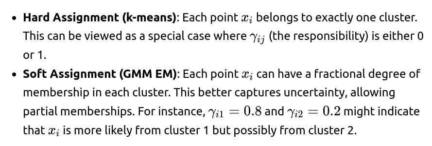
Soft assignment helps with more fine-grained cluster modeling, especially when clusters overlap or data has ambiguous cluster boundaries.

How can we incorporate priors or regularization into EM?

If you adopt a Bayesian perspective, you can impose priors on parameters like the means, covariances, or mixture weights. This modifies the M-step to maximize the posterior rather than the likelihood. For instance, you might have a conjugate prior for the Gaussian’s mean and covariance (e.g., Normal-Inverse-Wishart prior). Then the M-step becomes a maximum a posteriori (MAP) update. In practice, adding a Dirichlet prior on the mixture weights or a Wishart prior on the covariance can reduce overfitting and mitigate degenerate solutions (where a component collapses on a single point).

Why is the EM algorithm guaranteed to never decrease the observed data log-likelihood?

EM can be interpreted as coordinate ascent on a lower bound to the log-likelihood, or equivalently as the iterative optimization of the Evidence Lower BOund (ELBO). The E-step computes a distribution q(z) over latent variables that matches the posterior distribution of the latent variables given the data (using the current parameters). The M-step then updates the parameters θ to maximize the expectation of the complete-data log-likelihood under q(z). Each iteration is guaranteed not to decrease the log-likelihood because of Jensen’s inequality and the construction of the auxiliary function in the EM derivation. This ensures monotonic improvement or, in worst cases, maintains the same log-likelihood (e.g., at convergence).

Could you highlight a more advanced scenario where EM is used beyond simple GMM?

• Hidden Markov Models (HMMs): In HMMs, the latent variables are the hidden states at each time step. The E-step uses the forward-backward algorithm to compute the posterior of the hidden states, and the M-step re-estimates transition probabilities, emission probabilities, etc.

• Factor Analysis: Treat latent factors as unobserved variables that generate high-dimensional observations. EM can be used to iteratively infer latent factors and update loadings/covariance structure.

• Missing Data: When some features are unobserved for some data points, we can treat those unobserved features as latent variables. EM can be used to iteratively fill in (E-step) and update model parameters (M-step).

In all these contexts, the same pattern repeats: infer distributions over missing or hidden pieces of data, then optimize parameters given these distributions.

How do we handle the situation if k is unknown or if we suspect the data might not fit a standard GMM?

When k (the number of mixture components) is unknown, one can use methods such as:

• Model Selection Criteria: Evaluate results for different k using AIC (Akaike Information Criterion), BIC (Bayesian Information Criterion), or cross-validation. Then choose the kk that best balances goodness of fit with model complexity.

• Non-parametric Mixture Models (like Dirichlet Process Mixtures): Instead of fixing k, use a Dirichlet process prior to let the model infer the number of clusters from data. This still often involves variants of EM (or Gibbs sampling, variational inference) but is more flexible for discovering the appropriate number of mixture components.

For data that might not fit a standard GMM, people often try more flexible distributions or mixture-of-experts frameworks, or they might do transformations before applying a mixture model. Some use Gaussian mixture models as a starting point for clustering, but if the data is heavy-tailed or multi-modal in complicated ways, alternative distributions or mixtures (e.g., Student’s t-mixtures) can be more appropriate.

How do you ensure numerical stability in EM-based computations?

1. Log-space Computations: Avoid underflow when computing tiny probabilities by working in log space. For instance, when computing responsibilities, one can exponentiate differences of logs to maintain stability.

3. Check for NaNs: Implementation can break if log⁡(0) or division by zero is encountered. Good practice is to add small epsilons in denominators and logs.

4. Double Precision: Usually prefer double precision (float64) especially for complicated, long iterative processes.

If a GMM is high-dimensional, does EM still work?

EM still works but faces challenges in high-dimensional spaces:

• Covariance matrices become large (d×d if d is the dimension), leading to higher computational costs (inversion of large matrices can be slow or numerically unstable).

• Data sparsity can lead to poorly estimated covariance matrices. Regularization or dimensionality reduction might be necessary. One might also restrict to diagonal or low-rank covariance to manage complexity.

Nevertheless, the core procedure is the same: E-step (update responsibilities) and M-step (update parameters). Implementation details just become more complex for large d.

What if we want to do partial E or M updates instead of a full batch approach?

Online or incremental variants of EM exist. In large datasets, a full E-step and M-step on the entire dataset can be expensive:

• Online EM: Processes data in mini-batches, updating responsibilities for each mini-batch and then adjusting parameters accordingly. This can be viewed analogously to stochastic gradient descent but in an EM framework.

• Stochastic Variants: Combine ideas of variational inference and EM with smaller updates that yield faster iteration times at some cost to the final solution accuracy.

This is especially helpful when N (number of data points) is very large or arrives in a streaming fashion.

Summarizing Key Points Interviewers Look For

• Clear understanding of how the E-step infers the latent variables’ distribution.

• Ability to describe in detail how the M-step updates parameters to maximize the expected complete-data log-likelihood.

• Knowledge of typical pitfalls (local maxima, covariance degeneracies) and practical solutions (random restarts, regularization).

• Familiarity with real-world usage, e.g., GMM, HMM, missing data, factor analysis, and advanced scenarios like Bayesian or infinite mixture models.

• Awareness of how to implement EM and ensure numerical stability, correct convergence checking, and how to handle large or high-dimensional data.

---

Below are additional follow-up questions

Could EM be applied in a semi-supervised learning context where some labels or latent assignments are known and others are not?

In semi-supervised learning, we typically have a dataset where some observations have known labels (or partially observed latent variables) while others have no labels at all. The EM algorithm can be adapted to this scenario by treating the missing labels as latent variables and leveraging the known labels to guide the parameter updates.

For instance, suppose you have a Gaussian Mixture Model (GMM) with certain data points for which you already know their cluster assignments (these are “labeled”), and other data points for which the cluster assignment is unknown (these are “unlabeled”). In the E-step, you can fix the responsibilities for the labeled data to 1.0 for the known cluster and 0.0 for the others, while for unlabeled data you compute the responsibilities in the usual way. This partial observation of the latent variables constrains the solution space and often leads to better parameter estimates when data is scarce or noisy.

One subtle pitfall is that if you have too few labeled points, the guidance may be insufficient, and the EM algorithm could overfit to the partially labeled portion, failing to generalize well to unlabeled data. Conversely, if the labeled data contains outliers or mislabels, it could bias the parameter updates. Hence, it is important to have high-quality labeled data and possibly incorporate regularization or domain knowledge to mitigate these issues.

How does EM handle continuous latent variables, and does it differ significantly from discrete latent variable cases?

The conceptual framework of EM is the same regardless of whether the latent variables are discrete or continuous. In the discrete case (like in GMM where the latent variable is the cluster index), the E-step typically involves computing a discrete posterior probability distribution over each latent state. In the continuous-latent scenario (for example, in factor analysis models), the E-step requires computing a continuous posterior distribution.

If the posterior distribution over the continuous latent variable has a convenient form (e.g., a Gaussian in linear-Gaussian models such as factor analysis or probabilistic PCA), we can still obtain closed-form solutions for the E-step. Instead of “responsibilities,” we end up computing posterior means and covariances of the latent factors for each data point. Then, in the M-step, we update the model parameters by maximizing the expected complete-data log-likelihood under these posterior distributions.

A potential pitfall arises when the posterior over the latent variables is not tractable, as happens in more complex models (e.g., mixture of Gaussians plus some nonlinear transformations or in deep generative models). In those scenarios, the E-step might require approximate inference techniques, such as variational inference or Markov chain Monte Carlo sampling. EM can still be used in principle, but the “E-step” is replaced by an approximate inference procedure, leading to what is sometimes called a “Generalized EM” approach.

Can EM be used in a scenario where the data is not independently and identically distributed (i.i.d.), such as time-series data or correlated observations?

The classical EM algorithm typically assumes i.i.d. data for the derivation of the log-likelihood. However, we can generalize EM to handle non-i.i.d. structures by accurately defining the joint likelihood of all observations and latent states. Hidden Markov Models (HMMs) are a prime example: the observations are correlated over time, and the hidden states form a Markov chain. Yet EM is still employed via the Baum-Welch algorithm, which is a specialized version of EM for HMMs.

In time-series or correlated data scenarios:

• The “E-step” might involve running a forward-backward algorithm (in the case of HMMs) or a more complex inference procedure if the dependencies are richer.

• The “M-step” re-estimates the transition probabilities, emission probabilities, or other parameters that define the generative process over time.

One must be aware that strong temporal correlations can pose numerical challenges. For instance, if certain states or observations in an HMM become extremely unlikely, responsibilities can become numerically unstable. Implementing stable forward-backward recursions (often in log-space) is critical. In more general correlated models (like Dynamic Bayesian Networks), exact inference in the E-step can become intractable, requiring approximate methods or specialized dynamic programming.

Could EM be used with robust distributions to handle outliers or heavy-tailed data?

Gaussian Mixture Models can be sensitive to outliers because the Gaussian distribution has relatively thin tails. A few extreme outliers can drastically impact covariance estimates. One way to handle such scenarios is to replace the Gaussian components with heavier-tailed distributions, like Student’s t-distributions or Laplace distributions, so the model is more tolerant of extreme observations. The EM concept remains the same, but the E-step and M-step get derived from the new likelihood function.

For instance, using a Student’s t-mixture model can accommodate heavier tails. The presence of the additional degrees-of-freedom parameter in the Student’s t distribution modifies how responsibilities are assigned and how parameters are updated. Another approach is to apply data transformations or robust scaling before fitting a standard GMM.

A subtlety here is that with heavier-tailed distributions, the M-step can lose closed-form solutions. In such cases, you might need an iterative procedure (like Newton-Raphson) within the M-step. Also, if outliers are extremely severe, even heavier tails can fail to capture them properly, and you may have to adopt robust statistical methods that explicitly model outliers or use mixture components specifically dedicated to outlier “noise” clusters.

How might one parallelize or distribute the EM algorithm for very large datasets?

EM is traditionally a batch algorithm requiring access to all data in each E-step. For massive datasets, this becomes expensive or infeasible to do on a single machine. Several strategies exist:

• MapReduce-Style Summations: In the E-step, responsibilities for each data point can be computed in parallel across multiple workers. Each worker computes partial sums of responsibilities, partial sums for mean/covariance updates, etc. These partial results are then aggregated (e.g., a reduce step) to produce global sums. After that, the M-step uses these aggregated sums to update parameters.

• Online EM: Processes the data in mini-batches, updating parameters incrementally. Although strictly speaking, this modifies the standard batch EM algorithm, it is still recognized as a valid extension that can scale to large or streaming data.

• Distributed Memory Approaches: Frameworks such as Apache Spark or distributed HPC systems let you store the dataset across multiple nodes, compute the responsibilities locally, and synchronize the updates for each iteration.

Potential pitfalls:

• Synchronization overhead can be considerable if too many passes over the data are required.

• Convergence might become slower if updates do not see the entire dataset at once (as in online or mini-batch approaches).

• Numerical consistency can degrade if floating-point summations are done in different orders across distributed systems, leading to slightly different results from run to run.

What are the differences between “Generalized EM” and the standard EM algorithm, and why might we use the generalized version?

The standard EM algorithm requires a closed-form M-step or a complete maximization of the expected complete-data log-likelihood. In some models, an exact M-step is impossible or impractical because the optimization is too complicated. The “Generalized EM” (GEM) algorithm relaxes this requirement: instead of fully maximizing that expectation, you only need to increase it (i.e., perform a step that raises its value compared to the previous iteration).

For instance, you might do a single step of gradient ascent or apply a local numeric optimizer that runs for a few iterations without necessarily reaching the global optimum in each M-step. You still get monotonic increases in the data log-likelihood as long as the M-step ensures an improvement in that objective. This is common in complicated latent variable models, such as certain deep generative models, where partial or approximate updates in the M-step are more feasible than an exact solution.

One edge case is if your partial update in the M-step is too minimal, you risk very slow convergence or potentially stagnating. Another subtlety is ensuring the E-step is still done correctly, or in some approximations, that it too can be generalized (leading to variations often referred to as variational EM).

How do we decide when to stop EM iterations, and could early stopping be beneficial?

Common convergence criteria:

Early stopping can be beneficial if:

• Overfitting is suspected, especially in high-dimensional mixture models. When the model tries too hard to capture every nuance, it might start to cluster single points or produce near-singular covariances.

• You only need a “good enough” solution quickly. In large-scale or streaming applications, partial convergence might suffice, and those solutions can be refined when time and resources permit.

A subtlety is that you might stop too soon and miss a better local maximum. Monitoring a separate hold-out set’s log-likelihood (if possible) can provide a more robust gauge of overfitting or whether continuing to iterate yields real improvements.

How does EM compare to the Variational Inference (VI) approach in Bayesian latent variable models?

Variational Inference is another way to handle latent variable models, especially from a Bayesian perspective, where we place priors on parameters and aim to approximate the full posterior distribution. EM can be seen as a special case of coordinate ascent on the Evidence Lower BOund (ELBO) under certain assumptions, but in Bayesian settings, EM typically finds the mode of the posterior (i.e., MAP estimation) rather than the full distribution.

Variational Inference, by contrast, posits a family of distributions over latent variables and (possibly) parameters, then attempts to find the distribution within this family that maximizes the ELBO. This yields an approximation to the entire posterior, not just a point estimate. VI can handle more complex models, but might require more intricate derivations, and the resulting posterior approximations can be biased by the choice of the variational family.

A potential edge case is if the posterior distribution is highly multi-modal or skewed. Variational Inference might get stuck in a local maximum of the ELBO. EM, on the other hand, is also prone to local maxima. Which approach is best depends on how important capturing posterior uncertainty is and how tractable the model is with either method.

Does the EM algorithm have any guarantees about global convergence under certain conditions?

EM is known to guarantee that it will not decrease the observed data log-likelihood at each iteration, but in general, it is only guaranteed to converge to a local maximum, not necessarily the global maximum. However, there are special cases where the likelihood surface is convex in the parameters once the latent variables are integrated out, and thus EM can find the global optimum. A typical example is a single-component Gaussian with missing data that is missing completely at random. In more complicated mixture models, the function is non-convex, and multiple local maxima can exist.

A subtle point is that even if the complete-data log-likelihood is “nice,” once we marginalize out the latent variables for the observed-data log-likelihood, the objective can become non-convex. This is why mixture models, hidden Markov models, etc. often require careful initialization or multiple runs to find good solutions.

How does one handle mixture components that become redundant over time, for instance when one component ends up with very low responsibilities?

You might handle them by:

• Pruning them: If a component’s weight falls below a certain threshold, remove it. This adaptively reduces the number of components.

• Merging components that are too similar: After EM converges, if two components have very similar means and covariances, you might combine them into a single component with updated parameters.

A subtlety is that removing or merging components mid-EM can alter the overall log-likelihood surface. In principle, you might temporarily see a drop in the objective if not done carefully. A practical approach is to monitor if the model performance (via log-likelihood, AIC, BIC, or a validation measure) improves after such merges or pruning.

Could EM be used in an online learning or streaming context where data arrives sequentially?

Yes, there is an “online EM” algorithm that processes one (or a few) data points at a time. In online EM, each new data point triggers an E-step for just that data (or mini-batch), followed by a partial M-step update that moves parameters in a direction that would increase the expected complete-data log-likelihood. This approach is akin to stochastic gradient approaches, but within the EM paradigm.

Potential pitfalls include:

• Choosing a suitable learning rate or step-size schedule for the partial M-step is non-trivial. Too large a step can cause instability, too small leads to slow convergence.

• The model might be heavily influenced by the data order, especially if the data distribution shifts over time. Some form of forgetting factor or sliding window might be necessary if the data distribution evolves.

How do we incorporate constraints on parameters (e.g., forcing some means or covariances to be equal, or enforcing a low-rank covariance) in the EM algorithm?

Sometimes domain knowledge or computational constraints require certain parameter restrictions. For example:

• We might want all covariance matrices in a GMM to be diagonal or spherical.

• We might want certain means to remain fixed or tied together across components.

• We might require low-rank approximations for high-dimensional data to reduce computational cost.

In practice, you impose these constraints in the M-step by restricting the optimization to the feasible parameter space. For example, if you want a diagonal covariance, you only estimate the diagonal entries from the E-step responsibilities and keep off-diagonal entries zero. If some means must be identical across components, you would compute their updates by pooling responsibilities from all those components before computing a shared mean.

An edge case is that some constraints can make the maximum-likelihood problem degenerate. If you force too many constraints (e.g., zero covariance for a distribution that truly needs spread), the model can misfit the data, leading to poor log-likelihood. Another subtlety is that the closed-form M-step might vanish under certain constraints, forcing a more specialized numeric approach.

How might we debug or diagnose EM solutions if results look suspicious?

When an EM solution looks incorrect—perhaps because a component has collapsed or log-likelihood is not improving as expected—some debugging steps include:

• Check responsibilities: See if any component has near-zero or near-1.0 responsibilities for most data points. This can indicate collapsing.

• Visualize parameter updates: For GMMs in 2D or 3D, you can plot the current Gaussian ellipsoids and see if they match the data distribution.

• Ensure no data preprocessing or input errors: Verify data is scaled or standardized as intended. Large outliers or missing values can break assumptions.

• Look at log-likelihood at each iteration: If it’s oscillating or not increasing, there might be a bug in the E-step or M-step code. Possibly a dimension mismatch or a math error.

• Check for numeric underflow/overflow: If you are dealing with large dimension or extremely large/small data, do computations in log-space or add small values (epsilon) to denominators.

• Use simpler data: Start with a small synthetic dataset (like 2D points generated from known Gaussians) to see if the algorithm recovers the parameters as expected.

A subtlety is that visually suspicious solutions might actually be local maxima. The mixture might have latched onto a subset of data, ignoring the rest. Initializing from different random seeds or employing more robust initialization can help diagnose if a strange solution is a stable local mode.

How do we handle missing or incomplete feature values in a GMM using EM, distinct from the latent cluster assignments?

In practice, for each data point with missing features, we compute the sufficient statistics needed for the M-step by integrating over the distribution of the missing features. If the missing data pattern is not too complicated (e.g., missing completely at random and only a few features per data point are missing), we can still derive closed-form solutions. If it’s more complex, approximate methods might be necessary.

A subtlety is that if the fraction of missing data is extremely high, the constraints on parameters from the partially observed data might be insufficient, leading to identifiability issues. Another subtlety is that the mechanism of missingness (missing completely at random vs. missing at random vs. missing not at random) can drastically affect how the E-step should be formulated, which can complicate the application of EM.

How does regularization or prior knowledge about the parameters get integrated into EM beyond simply adding a diagonal term to covariances?

Regularization can be introduced by placing priors over the parameters and then turning the likelihood maximization into a posterior maximization (MAP-EM). For a GMM:

• A Dirichlet prior on the mixture weights biases them away from extremes (0 or 1).

• A Normal prior on the means shrinks them to a central location.

• An Inverse-Wishart prior on covariances encourages certain shapes or magnitudes.

In practice, the M-step becomes maximizing the log posterior (the sum of log-likelihood and log prior). For standard conjugate priors (like Normal-Inverse-Wishart), the parameter updates might still be partly analytic. For more complex priors, numeric methods or partial M-step updates are necessary.

An edge case is that if the prior is too strong (e.g., very tight around certain means or covariance values), you may overshadow the actual data evidence. Conversely, if the prior is too weak, you gain little advantage. Another subtlety is that if your prior is incorrectly specified, it can systematically bias parameter estimates. Tuning hyperparameters for these priors is often just as important as choosing the number of components.

How can we adapt the EM algorithm for discrete data models (e.g., mixture of categorical distributions) and what unique pitfalls may arise?

For discrete data where each feature is categorical, we might use a mixture of multinomial or Bernoulli components instead of Gaussian components. The EM structure remains:

• E-step: Compute posterior probabilities (responsibilities) that each mixture component generated each observed discrete vector.

• M-step: Update the parameters of each discrete distribution (like probabilities of each category within each mixture component) by using those responsibilities as weights.

Unique pitfalls:

• If any particular category never appears in the data assigned (even fractionally) to a component, the parameter for that category might get stuck at zero, and subsequent EM iterations might never assign future data to that component if the distribution is strictly zero for that category. Smoothing or pseudocounts (like Laplace smoothing) can mitigate this.

• If the data has many categorical features, the parameter space can be huge, and the mixture model can be extremely flexible, risking overfitting. You may need to reduce dimensionality, tie parameters across categories, or introduce a hierarchical prior for smoothing.

A subtlety is that these discrete mixture models can be more prone to local maxima if certain components latch on to small subsets of the data. Proper initialization (e.g., from a simpler clustering approach or domain-based initialization) is crucial to avoid degenerate solutions.

How might EM be extended or adapted to simultaneously learn model hyperparameters (e.g., the number of mixture components k) without a separate model selection procedure?

One approach is to treat k itself as a random variable in a nonparametric Bayesian framework, such as a Dirichlet Process Mixture Model, which can be implemented with methods akin to EM (though typically Gibbs sampling or variational inference is used). Another strategy is the reversible-jump MCMC approach, but that’s beyond pure EM.

A subtlety is that algorithms that re-estimate k on the fly risk merging or splitting components in a single iteration, which is not part of classical EM. This leads to “birth-death” processes or “merge-split” moves that go beyond standard E and M steps, so it is more of a specialized extension than a straightforward application of EM.

How do we handle label switching or identifiability issues in mixture models?

Mixture models exhibit a fundamental label switching ambiguity: permuting component labels (e.g., swapping component 1 with component 2) yields the same overall likelihood if the parameters are swapped accordingly. This is not inherently a problem for the likelihood, but it can complicate interpretation. If you run EM multiple times, the order of learned components can differ, which is not a bug but a known identifiability issue.

When you need interpretability (e.g., cluster 1 should correspond to a specific known subpopulation), you might fix certain constraints, such as ordering the component means after each iteration so that they are sorted by their first dimension or by their mixture weight. Alternatively, you can post-process the final solution to reorder components in a consistent manner.

A subtlety is that if two clusters are extremely similar, label switching might happen mid-training, giving the impression that parameters “jump around.” This can create non-smooth training curves if you track per-component metrics. However, from a purely likelihood standpoint, it makes no difference.

How does EM interact with model-based outlier detection or novelty detection?

In model-based outlier detection, you typically fit a density model (such as a GMM) to normal data, then label points as outliers if their likelihood under that model is below some threshold. If you attempt to incorporate outliers into the training set, they can skew the parameter estimates of the mixture. Some advanced methods introduce a special “outlier component” that has a broad distribution. The E-step will assign high responsibility of outlier points to that special component, preventing them from distorting the core clusters.

Pitfalls include:

• If outliers are not too extreme, they might partially distort the main components instead of being assigned to the outlier component.

• If the outlier fraction is large, the model might interpret them as legitimate clusters.

• Tuning the outlier component’s parameters or deciding how to enforce a minimal or maximum fraction of outliers can be tricky.

A subtlety arises if the boundary between “normal” and “abnormal” data is not well-defined. EM cannot solve that conceptual problem on its own. You may need domain-specific thresholds or additional constraints.

How do we interpret negative log-likelihood values when diagnosing EM performance?

Because GMM log-likelihoods (or any mixture log-likelihood) can be negative, it is often more practical to track the negative log-likelihood (NLL) and see if it is decreasing over EM iterations (which corresponds to the original likelihood increasing). Large negative values do not necessarily indicate a bad model if the dimension of data is high or if the scale of the variables is large, because the Gaussian density function can be very small.

Comparing absolute NLL values across different transformations or rescalings of data can be misleading unless done carefully. What matters is the relative improvement from iteration to iteration (or between models). Also, if you are comparing GMMs with different k, you might need criteria like BIC or AIC, or cross-validation, to account for changes in model complexity.

A subtlety is that if you add regularization terms or if you do a MAP-based approach, you are no longer purely optimizing the negative log-likelihood but a sum of negative log-likelihood and penalty/ prior terms. Hence the interpretability of the scale changes. You must keep track of whether you are measuring just the data likelihood or the posterior.

How can we adapt the E-step in large mixture models if it becomes a bottleneck?

In the E-step, for each data point you compute responsibilities with respect to each of the k mixture components. This is O(N×k) in naive form. If N is huge and k is large, this can be computationally expensive.

Potential strategies:

• Approximate Nearest-Cluster Search: If you expect many components to have negligible probability for a given point, you can skip or approximate their responsibilities. A clustering data structure or tree-based approach can quickly identify the few most relevant components.

• Coresets or Subsampling: You might do the E-step on a subsample of data or use existing responsibilities as an approximation for “similar” data points in the next iteration.

• Hierarchical Mixture: You could represent the mixture as a tree, so the E-step visits broad mixture partitions first, then refines the responsibilities only within relevant subtrees.

A subtlety is that approximations can degrade the exactness of the EM updates, potentially slowing or destabilizing convergence. Careful balancing of speed gains and accuracy loss is required, especially if you rely on the resulting model for critical tasks like anomaly detection or risk scoring.

How does one interpret responsibilities in a real-world application, and do they correspond to a probability of membership in a strict sense?

In practice, the model might be approximate, some components might be overlapping, or the data might contain structure not captured by the mixture. Responsibilities then become a relative measure of how well each component explains each data point, rather than an absolute probability that can be taken at face value.

A subtlety is that if certain clusters have near-identical parameters, the distribution can be nearly degenerate, and responsibilities might become numerically unstable or flick between these identical clusters. Another subtlety is that in truly high-dimensional spaces, it can be hard to interpret responsibilities, as many data points may have very diffuse membership across components if the data is not well-clustered.

How does the variance of the estimate from EM compare to the variance if we had a fully observed likelihood?

In a latent variable setting, we are missing part of the data. The maximum-likelihood estimates will typically have higher variance (i.e., more uncertainty in the estimated parameters) compared to if we had directly observed the latent variables. EM finds a point estimate, but it does not directly give you confidence intervals or distributions over parameters.

If you want uncertainties, you can resort to:

• Observed Information Matrix or Louis’ Formula to approximate the Fisher Information in incomplete-data scenarios, though it can be intricate to compute.

• Bootstrap approaches: run EM multiple times on resampled data to see the variability in the parameters.

A subtlety is that for some models, the missing data can drastically degrade identifiability. You might end up with large confidence regions for certain parameters or an inability to separate multiple mixture components effectively. Another subtlety is that the EM iteration itself does not produce a covariance estimate for parameters by default; you must do additional computations or rely on approximate methods post hoc.

How can EM be adapted for mixture of experts or gating networks?

A mixture of experts extends GMM-like ideas to regression or classification contexts, where each “expert” (component) is a conditional model (like a linear or logistic regression) rather than a Gaussian density. A gating network outputs mixture weights. The E-step remains: compute responsibilities that each expert is responsible for a given data point’s output. The M-step updates the parameters of the experts and the gating function.

For a simple mixture of linear regressions, the responsibilities for each data point can be computed from the predicted likelihood under each linear model times the gating weight. Then you re-estimate regression coefficients in the M-step using a weighted least-squares. A subtlety is that if the gating network is also parameterized (e.g., a softmax function of some gating parameters), you need to do a separate M-step for those gating parameters, typically requiring gradient-based optimization. Another subtlety is that if experts share hidden layers (as in neural networks), the M-step might require backpropagation, which merges EM with gradient-based updates.

Could one combine EM with neural networks in a hybrid model, and what are key challenges?

Yes. For example, in some architectures, you might have a latent variable that is partially encoded by a neural network. The E-step would then require computing the distribution over that latent variable given the current network weights, and the M-step would update the network weights to maximize the expected complete-data log-likelihood. This might be akin to the wake-sleep algorithm in Helmholtz machines or certain forms of variational autoencoders that incorporate an EM-like approach, though VAEs typically use differentiable approximations rather than a pure EM structure.

Key challenges:

• The E-step might not be analytically tractable if the neural network is complex. Approximate inference is needed.

• The M-step might require gradient-based methods if no closed-form solution exists. This is effectively a Generalized EM approach.

• Large-scale training can be slow if you combine iterative EM with the already high computational cost of neural networks.

A subtlety is that the synergy between neural network function approximators and EM’s iterative nature can lead to better local minima or can cause optimization instability if not managed carefully (e.g., step sizes, regularization, or approximate E-step accuracy). Another subtlety is that if the neural network is over-parameterized, you might need strong priors or constraints to avoid degenerate solutions.

How do we handle domain-specific constraints or interpretability requirements in an EM-based approach?

In many real-world applications—medical imaging, finance, biology—there may be domain constraints, like certain parameters must remain within a physically meaningful range, or certain latent variables must reflect real attributes (e.g., different tissue types in an image). You can incorporate these constraints by:

• Adding penalty functions or priors that restrict parameters to plausible ranges.

• Forcing certain mixture components to represent known subpopulations with partially fixed parameters (semi-supervised or constrained EM).

• Post-processing the EM results to discard or merge solutions that do not align with domain understanding.

A subtlety is that imposing domain constraints might break some of the neat closed-form updates. You might need to project parameters back to the constrained set after each M-step or use partial numeric optimization. Another subtlety is that interpretability can conflict with purely data-driven solutions if the data suggests a different structure than the domain constraints permit.

How would we validate an EM-based clustering solution if we don’t have ground-truth labels?

Clustering validation without ground-truth labels can rely on:

• Internal measures like silhouette score or the negative log-likelihood itself.

• Stability-based measures: run EM multiple times with different seeds or subsets of data, then see if you get consistent solutions.

• Information criteria like BIC and AIC to penalize model complexity.

A subtlety is that the best “internal measure” might not align with domain-specific utility. For example, a particular mixture might yield a better negative log-likelihood but be less interpretable or might not align with known subcategories in the application domain. Another subtlety is that for high-dimensional data, many standard clustering metrics can become less meaningful, requiring specialized metrics or dimension reduction for interpretability.

How do we incorporate external side information (like labels for a subset of features or domain heuristics) into an EM-based cluster or mixture model?

You might treat side information as partially observed latent variables or as constraints in the likelihood function. For example, if you know that certain data points must be in the same cluster, you could modify the responsibilities in the E-step to enforce that. Alternatively, you could create a prior distribution that correlates data points with known side information to the same component.

Edge cases arise if the side information conflicts with what the raw data implies. The EM algorithm can become stuck trying to reconcile contradictory constraints. Another subtlety is that side information might be uncertain or noisy, in which case you treat it as an additional probabilistic component in the E-step. This complicates the model but can significantly improve clustering accuracy if done properly.

How might we handle multi-modal distributions that each require multiple Gaussian components, and ensure we’re not over-splitting or under-splitting clusters?

If you have multiple separated modes in the data, you might need more than one component per mode if the shape in each region is not perfectly elliptical. The question is whether to use a single large covariance Gaussian to model each mode or multiple smaller Gaussians.

One approach is hierarchical mixture modeling: first partition the data into broad modes, then apply a sub-mixture to each mode. Alternatively, a large k might naturally let EM place multiple Gaussians in each mode. One must watch for overfitting if k is too big. Criteria like BIC or cross-validation can guide the choice of k or the hierarchical structure.

A subtlety is that if different modes overlap slightly, the algorithm might put a single Gaussian bridging them, leading to a poor fit overall. Another subtlety is that sometimes a single Gaussian per mode is enough if the data is roughly elliptical in each mode; if it’s not elliptical, multiple Gaussians might fit better but at the risk of over-segmentation.

What if the data truly follows a mixture distribution with correlated components, can EM still handle that?

If by “correlated components” you mean that the latent variables themselves are correlated, a simple mixture model might not suffice because it assumes each data point is generated independently from a single mixture component. You could introduce hierarchical structures or nested latent variables that capture correlations among components. Each approach can still be framed in an EM-like framework but with a more complex joint probability.

A subtlety is that once correlation among latent variables is introduced, the standard factorized form used in typical mixtures no longer applies, and the E-step might become intractable. One might need approximate inference, such as variational methods. Another subtlety is that correlated mixture components could be better captured by fewer but more flexible distributions, or by a high-level latent variable controlling correlation across mixture membership.

Below are additional follow-up questions

What if the data distribution changes over time (concept drift)? How would we adapt EM in a non-stationary setting?

In real-world scenarios like streaming data or continuous monitoring systems, the underlying data distribution can change over time (also known as concept drift). Standard EM assumes a fixed data distribution. If the distribution shifts significantly, the learned model parameters can become outdated.

To handle concept drift, a few strategies can be used:

• Sliding Window or Forgetting Factor: One approach is to re-run EM on the most recent batch of data, discarding old observations or gradually down-weighting them. This ensures that the model parameters reflect the current distribution. A sliding window approach might keep only the last ( N ) data points and periodically re-estimate parameters. A forgetting factor approach updates responsibilities in the E-step but discounts older data by a factor ( \alpha < 1 ).

• Online or Incremental EM: Instead of running standard EM in large discrete iterations, one can process small batches (or individual observations) as they arrive. After each batch, the algorithm updates responsibilities and parameters. This incremental approach can be adapted so that recent data has a stronger effect on the parameter updates.

• Adaptive Mixture Components: If new modes appear in the distribution or existing modes disappear, a fixed number of Gaussian components may no longer be sufficient. One could dynamically add or remove mixture components based on model selection criteria (e.g., penalized likelihood, minimum description length) or based on a threshold of “unexplainable” new data.

A potential pitfall in concept-drift scenarios is that large, sudden changes can cause catastrophic forgetting, where the model overfits to recent data and completely loses the structure learned from older data. One must balance responsiveness to new patterns with retention of historical knowledge.

How does EM behave in the presence of outliers or heavy-tailed data?

When the data has extreme outliers or follows a heavy-tailed distribution, a Gaussian Mixture Model (with standard covariance assumptions) may be too sensitive to these extreme observations. During the M-step, the maximum likelihood covariance can become inflated if outliers fall far from the means, causing the algorithm to assign them a small but non-negligible probability spread across multiple components.

Common solutions and considerations:

• Robust Mixture Models: Instead of using standard Gaussian components, one can use mixture models with heavier-tailed distributions like Student’s t-distributions. This naturally reduces the impact of outliers because t-distributions can accommodate heavier tails.

• Regularizing Covariance Updates: Adding a small regularization term (e.g., a diagonal value (\lambda I)) during covariance updates can prevent singularities or extreme expansions of the covariance.

• Trimmed EM: A technique that down-weighs or even discards data points that have very low responsibility under all components (i.e., “extreme outliers” that do not belong to any cluster). This approach can keep the parameter estimates from being disproportionately influenced by a small number of anomalies.

A subtle issue arises if outliers contain significant information about a rare subpopulation in the data. Filtering out outliers might lose genuinely meaningful structure. Careful domain knowledge is often needed to decide which approach is best.

How do we decide on the number of mixture components in a GMM, and how does EM handle this?

Choosing the correct number of components (k) is a major challenge in mixture modeling. EM itself only performs parameter estimation given (k); it does not automatically determine the best (k). If (k) is too large, the model might overfit. If (k) is too small, the model might fail to capture all subgroups.

Strategies for choosing (k):

• Information Criteria: The Bayesian Information Criterion (BIC) or Akaike Information Criterion (AIC) penalizes model complexity. One can train multiple GMMs with different (k) values, compute BIC or AIC, and select the (k) that yields the best trade-off between fit and complexity.

• Cross-Validation: Splitting the dataset into training and validation sets, one can evaluate log-likelihood on the validation set for various (k) and pick the best performer.

• Hierarchical / Dirichlet Process Mixtures: More advanced Bayesian techniques like the Dirichlet Process Mixture Model treat (k) as effectively unbounded and let the data guide how many components are needed. However, this requires more complex inference methods (e.g., variational or sampling approaches), which go beyond standard EM.

A pitfall is that the EM solution for a given (k) can converge to a local maximum that might differ for different initializations. Even if you run BIC or AIC over different (k), it might be biased by the starting parameters. A robust approach is to run multiple initializations and pick not only the best (k) but also the best local solution for each (k).

What is the role of partial or incomplete observations in EM, and how is it handled differently compared to missing latent variables?

In many real scenarios, not all features of a data point are observed. For example, you might have a dataset where some attributes are missing or uncollected. This differs from the presence of a fully unobserved latent variable like “component membership” in GMM. The principle of EM can still apply, but the notion of “E-step” includes inferring the distribution of missing features given the observed ones and current parameters.

For each data point:

• E-step: Compute the conditional distribution of missing features (and possibly latent class membership if it’s also relevant) given the observed features and current model parameters. • M-step: Update parameters by maximizing the expected complete-data likelihood with respect to that conditional distribution of the missing attributes.

Subtle pitfalls:

• Informative vs. Random Missingness: If the data is missing not at random (MNAR), standard EM assumptions (that the missingness is independent of the unobserved values) may be violated. This can bias parameter estimates. • High fraction of missing data: If a large portion of each data point is missing, the E-step’s distribution can become extremely uncertain, leading to potential instability. Additional constraints or priors might be needed to stabilize the solution.

How does one handle constraints like requiring each component’s covariance to be diagonal or tying certain parameters across components?

Sometimes domain knowledge or computational constraints dictate that each Gaussian’s covariance matrix must be diagonal (no off-diagonal correlations), or that all components share the same covariance structure. This can simplify calculations significantly (covariance inversions become trivial in the diagonal case) and also reduce the risk of singular matrices.

In the M-step, these constraints change how we maximize the expected complete-data log-likelihood. For diagonal constraints, one would only update the diagonal entries of the covariance. For tying constraints (e.g., all covariances are the same but differ in means), the single covariance is updated by pooling responsibilities across all components:

• Unified Covariance: Summation over all components’ responsibilities is aggregated before computing a common covariance. • Diagonal Covariance: Off-diagonal terms are set to zero. We only update the variance of each dimension independently.

Pitfalls include the possibility of underfitting if the actual correlations between features are strong. Imposing too many constraints can lead to a model that cannot capture the true data structure. On the other hand, in high-dimensional settings with limited data, these constraints can prevent overfitting and instability.

Could the EM algorithm be used if our mixture components themselves are not Gaussians?

Yes. EM is a general approach to maximum likelihood or MAP estimation with latent variables. The mixture components can be any parametric family: multinomials, Poisson, or more general exponential family distributions. The procedure remains:

1. E-step: Compute posterior responsibilities that each latent component generated a given data point, based on the current parameters and the data likelihood.

2. M-step: Update the component parameters by maximizing the expected complete-data log-likelihood under those posterior responsibilities.

The biggest difference is that the formula for the M-step changes based on the assumed family of distributions. For instance, if the mixture components are Poisson, the mean parameters of the Poisson components would be updated using the responsibilities. If the mixture components are Beta distributions (for some Beta mixture), the shape parameters would be updated accordingly.

A subtlety is whether each family admits closed-form solutions in the M-step. If not, one might need a numerical optimization step for each component. But the overarching EM procedure still holds.

How can we interpret convergence quality, and are there any post-hoc checks to verify if EM got stuck?

Once EM converges, typically we’ve found at least a local maximum. But the final solution’s quality can be evaluated in a few ways:

• Log-likelihood Plateau: If the observed log-likelihood has leveled off, that indicates numerical convergence. • Multiple Random Restarts: Run EM multiple times with different initial seeds. If multiple runs yield similar solutions, one can be more confident about the quality. If they produce significantly different solutions, it suggests multiple local maxima. • Cluster Quality Metrics: If using EM for clustering (e.g., GMM for cluster assignments), metrics like the silhouette coefficient, Dunn index, or Davies–Bouldin index can evaluate the separation of clusters. • Visual Inspection: With low-dimensional data (or reduced dimensional projections), one can visually check whether the clusters formed are sensible and whether the responsibilities appear stable.

A hidden pitfall is “false convergence” where the algorithm seems to stop changing because of numerical precision issues (very tiny updates) or because a covariance has become nearly singular, leading to instability. One might need to watch for extremely small or large parameter values that indicate numerical anomalies.

In high-dimensional data, does EM remain feasible, or how might we adapt it?

High-dimensional data poses unique challenges:

• Covariance Estimation: Computing and inverting a full covariance matrix is (O(d^3)) for (d)-dimensional data. If (d) is very large, this becomes prohibitive. Also, estimating so many parameters reliably requires a large dataset, risking overfitting. • Regularization: A common approach is to assume diagonal or low-rank covariances, or to apply shrinkage methods that ensure numerical stability and reduce variance in parameter estimates (e.g., (\text{cov}_j + \lambda I)). • Dimensionality Reduction: One might first apply PCA or another dimensionality reduction technique to reduce (d) to a more manageable dimension, then fit a GMM or another mixture model in the reduced space. • Sparse Modeling: Another advanced approach is to impose sparsity constraints on covariance or inverse covariance. This requires specialized versions of EM that incorporate regularization into the M-step.

Pitfalls include losing interpretability when heavily regularizing or reducing dimensionality. Also, if the intrinsic data structure is fundamentally high-dimensional, dimension reduction could discard important information.

Are there scenarios where a Generalized EM algorithm (GEM) is used instead of the standard EM?

Yes. Generalized EM relaxes the requirement that the M-step must fully maximize the expected complete-data log-likelihood. Instead, it only requires that the M-step achieve a non-decreasing update. So one might use a single gradient-ascent iteration or another partial optimization approach.

Scenarios where GEM might be preferred:

• Complex Models: If the parameter space is large or the likelihood is complicated, a closed-form M-step is not available, and performing a full numerical maximization might be too expensive per iteration. A partial improvement each iteration can still guarantee that the overall likelihood does not decrease. • Constraints or Regularizers: If the M-step includes constraint satisfaction or advanced regularization, an iterative sub-optimization can be run for a fixed number of steps. This partial approach still moves the parameters “upwards” in likelihood space, fulfilling the GEM property.

A subtle edge case arises if the partial M-step does not sufficiently increase the expected log-likelihood. If the step size is too small, convergence can be exceedingly slow, or the algorithm might get stuck in a shallow region of parameter space. Tuning these partial optimization methods can be tricky.

How can we use EM to deal with out-of-distribution or new classes in clustering tasks?

If applying GMM clustering via EM, the model is limited to the existing set of (k) mixture components. In many real-world applications, novel structures or “new classes” might appear that were not initially present:

• Model Misspecification: If the data has a new modality or cluster that does not match any existing component, the algorithm will force-fit those new points into one of the existing (k) Gaussians. This can degrade cluster quality. • Adaptive Mixture Model: One approach is to dynamically add a new Gaussian component when the data points consistently do not match well with any current component’s responsibilities. However, this typically requires more advanced Bayesian or heuristic expansions of the mixture model. • Rejection Mechanism: In some applications, you might add an “outlier” component or a “background” distribution. If certain data points have a probability below a threshold for all known components, they get assigned to a special outlier class. This does not solve the problem of discovering a new class but at least flags such data as unexplainable by the current mixture.

An edge case is if the new data truly belongs to a new distinct distribution that is quite different from all existing components. Without a mechanism to expand (k), standard EM-based GMM cannot spontaneously represent that cluster well.

How do we incorporate domain knowledge into an EM-based approach?

Often, purely data-driven EM might not capture domain nuances. Domain knowledge can be injected in multiple ways:

• Informative Priors (Bayesian EM): If we know that means or covariances should not deviate too far from certain values, we can use conjugate priors in a Bayesian or MAP framework. The M-step then becomes the mode of the posterior rather than the likelihood alone. • Constraints on Parameters: If domain experts say that certain clusters must share the same mean or that certain covariance structures should be identical, this drastically reduces the parameter space, guiding the algorithm toward physically plausible solutions. • Partial Labeling: If partial labels for cluster assignments are available, those can be treated as “observed” latent variables. The E-step is then only for unobserved data points. This can help anchor the parameter estimates to ground truth in some parts of the dataset.

A subtle pitfall is injecting domain knowledge that conflicts with the actual data patterns. This can lead to systematically biased estimates. One must balance domain knowledge with the model’s capacity to learn from data.

How can EM be combined with neural network approaches?

Although EM is traditionally discussed in the context of simple parametric models like GMM or HMM, there are hybrid approaches:

• Mixture Density Networks: A neural network outputs the parameters of a mixture distribution (e.g., mixture of Gaussians). In principle, one could interpret part of the network as generating mixture parameters, and apply an EM-like procedure to refine latent assignments. However, the typical approach is to train the network by backpropagation on the negative log-likelihood of the mixture distribution directly (i.e., no explicit EM steps). • EM as a Layer: In some specialized architectures, an EM or iterative inference step is included as part of the computational graph. Then the entire pipeline can be trained end-to-end. This can be seen in certain amortized inference methods for latent variable models, but it complicates the parameter updates since one might combine gradient-based learning with iterative expectation-maximization. • Deep Generative Models: Methods such as Variational Autoencoders (VAEs) use variational inference rather than EM. However, both frameworks (EM and VI) are conceptually related in that they approximate or optimize a lower bound on the log-likelihood.

Pitfalls include significantly increased implementation complexity and possible instability if the iterative EM updates conflict with standard gradient-based optimization steps. Careful scheduling or synergy between the two is needed to avoid a tug-of-war in the parameter space.

Under what conditions might we prefer sampling-based methods (like MCMC) over EM?

For complex latent variable models with highly multi-modal posteriors, or where the distributions are not well-approximated by simple parametric updates, sampling-based methods (e.g., Markov Chain Monte Carlo) might be preferred:

• Multi-modal Posteriors: EM converges to a single mode (local maximum). MCMC, in theory, can explore multiple modes by sampling from the posterior. • Non-Conjugate / Complex Models: If the model’s structure or priors lead to no closed-form solutions in the M-step and complicated objective surfaces, MCMC can directly sample from the joint parameter-latent space without needing closed-form partial updates. • Exact vs. Approximate: EM is effectively a point-estimate approach (maximum likelihood or MAP). MCMC can provide a full posterior distribution over parameters, which might be valuable for uncertainty estimation.

A drawback to MCMC is that it can be computationally expensive and tricky to diagnose convergence. Meanwhile, EM can be faster for problems like GMMs where each iteration has straightforward analytic updates. Another subtlety is that MCMC can get stuck in certain modes or suffer from poor mixing if the target distribution is highly dimensional or correlated, so it is not a panacea.

How do we prevent or detect numerical issues like underflow or overflow in the E-step for large datasets?

In the E-step of GMM, we compute probabilities that can become very small if the data dimension is large or if certain points lie far from the mean. Summing or multiplying these tiny probabilities can cause numerical underflow, leading to responsibilities being computed as 0 or NaN. Conversely, if data matches a component very strongly, exponent terms might overflow.

Typical approaches:

• Log-Sum-Exp Trick: Instead of computing probabilities directly in linear space, maintain everything in log-space and use the numerically stable log-sum-exp function to avoid underflow/overflow. • Scaling: In each iteration, find the maximum exponent among all components for a given data point and subtract it before exponentiating. This normalizes the likelihoods to a manageable numerical range. • Check for NaNs: Implement safety checks that detect if parameters become NaN or Inf. If that happens, one might re-initialize or reduce the step size in the M-step (in a generalized EM scenario).

A subtle pitfall is misapplying the log-sum-exp trick and introducing unexpected offset biases. Thorough testing and debugging are crucial in high-dimensional or large-scale data contexts.

How would you modify EM if the data was partially labeled or if we had semi-supervised data?

In semi-supervised setups, some data points come with known latent assignments (e.g., known cluster labels), while others are unlabeled. The E-step can be adapted so that the responsibilities for labeled points are fixed at 1 for the known component (and 0 for others), whereas unlabeled data points have responsibilities computed in the usual way. The M-step then incorporates both the fixed responsibilities from labeled data and the inferred responsibilities from unlabeled data.

Advantages:

• Improved Parameter Estimation: The presence of labeled points can guide the mixture components in the right direction. • Faster Convergence: The algorithm has partial knowledge that helps reduce the space of solutions.

Edge cases or pitfalls:

• Incorrect Labels: If the partial labels are noisy or incorrect, they can bias the entire model. The EM procedure trusts the labeled assignments, so the resulting parameters might systematically deviate. • Imbalance: If the labeled set is not representative (e.g., it comes mostly from one cluster), the model might underfit the unlabeled clusters. One might need to weight the labeled data differently or carefully ensure it is representative.

How do we handle a scenario where some mixture components collapse to a single point or vanish?

During EM, especially with GMMs, you may find a component’s covariance approaches zero or its mixture weight approaches near zero:

• Singularities: A Gaussian with nearly zero covariance at a single data point yields an infinite likelihood for that point, but this is not a useful global solution. • Vanishing Components: If responsibilities for a particular component remain extremely small for all data points, the mixture weight might fall near zero, effectively removing that component from the model.

Possible strategies:

• Minimum Variance Constraint: Impose a floor on the covariance eigenvalues to prevent singularities. • Component Resetting: If a component’s weight falls below a threshold, re-initialize it to a different region with random points or domain-driven guesses, trying to rescue it from vanishing. • Regularization: Add a prior that prevents extremely small or large mixture weights, or that penalizes very tight covariances.

A subtle consideration is whether a collapsed component might actually indicate meaningful structure in the data (e.g., extremely tight cluster). Typically though, it indicates an overfitting scenario or insufficient data to maintain a broad distribution for that component.

Does EM produce confidence intervals or uncertainty estimates for the parameters?

Standard EM provides point estimates of model parameters that maximize the likelihood. It does not directly yield uncertainty intervals or Bayesian credible intervals. However, there are ways to approximate or extend EM for uncertainty quantification:

• Observed Fisher Information: One could attempt to approximate the variance of the parameter estimates via the observed information matrix at the final EM solution. This approach can be mathematically involved and not always straightforward to implement. • Parametric Bootstrap: After EM converges, one can sample synthetic datasets from the fitted mixture model, re-run EM on each synthetic dataset, and look at the variability in the resulting parameter estimates. This bootstrap approach approximates the confidence regions. • Bayesian Extensions: A fully Bayesian approach (using priors and performing posterior sampling or variational inference) can provide natural uncertainty estimates, albeit at greater computational cost.

A caution is that naive confidence interval approximations might understate or overstate uncertainty if the model has multiple modes or if the data is limited. The shape of the log-likelihood landscape can be quite complex.

Could EM be used for tasks like density estimation or anomaly detection?

Yes, after fitting a GMM (or another mixture model) via EM, one obtains a complete parametric estimate of the density. This can be used for:

• Density Estimation: For any new point ( x ), evaluate ( p(x) = \sum_{j=1}^k \pi_j \mathcal{N}(x \mid \mu_j, \Sigma_j) ). That value indicates how likely ( x ) is under the learned distribution. • Anomaly Detection: Points with very low density ( p(x) ) can be flagged as anomalies. Alternatively, one can examine the posterior responsibilities to see if the point does not reasonably fit any particular component.

Pitfalls in anomaly detection:

• High-Dimensional Data: Densities can be extremely small even for “normal” points in high dimensions, complicating threshold selection. • Model Misspecification: If the mixture distribution does not match reality (e.g., data is not well described by Gaussians or the chosen number of components is insufficient), the resulting density estimate might mislabel normal points as anomalies. • Non-Stationary Environments: If the data distribution changes over time, the GMM might need continuous updates or risk labeling new normal behaviors as anomalies.