
ML Interview Q Series: Expected Distance on Unit Circle Circumference via Parametric Integration
Browse all the Probability Interview Questions here.
Let ((X,Y)) be a randomly chosen point on the circumference of the unit circle having ((0,0)) as center. What is the expected length of the line segment between the points ((X,Y)) and ((1,0))?
Short Compact solution
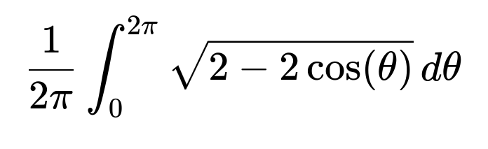
We note that if ((X,Y)) lies on the unit circle, then (X^2 + Y^2 = 1). The distance from ((X,Y)) to ((1,0)) is (\sqrt{(X-1)^2 + Y^2}). Since (X) can be expressed as (\cos(\Theta)) for a uniformly distributed (\Theta) on ((0, 2\pi)), we can write the expected value as the following integral:
Evaluating this (either analytically or numerically) shows that

which also simplifies to (4 / \pi).
Comprehensive Explanation
Deriving the distance formula
A point ((X,Y)) on the unit circle satisfies:
(X^2 + Y^2 = 1)
We want the distance between ((X,Y)) and ((1,0)). Denote this distance by (L). Then:
(L = \sqrt{(X - 1)^2 + Y^2})
Since ((X,Y)) lies on the unit circle, let (X = \cos(\Theta)) and (Y = \sin(\Theta)), where (\Theta) is uniformly distributed over ([0, 2\pi]). Substituting these into the distance formula:
(L = \sqrt{(\cos(\Theta) - 1)^2 + \sin^2(\Theta)})
Expand and simplify:
((\cos(\Theta) - 1)^2 = \cos^2(\Theta) - 2\cos(\Theta) + 1)
and
(\sin^2(\Theta) = 1 - \cos^2(\Theta)).
Hence,
[
\huge L = \sqrt{\cos^2(\Theta) - 2 \cos(\Theta) + 1 + 1 - \cos^2(\Theta)} = \sqrt{2 - 2\cos(\Theta)}. ]
Expected value of (L)
Because (\Theta) is uniform on ([0, 2\pi]), the expected value of (L) is

One can evaluate this integral either by:
A direct trigonometric approach with substitutions (e.g., using the identity (1 - \cos(\theta) = 2 \sin^2(\theta/2))), or
Numerical integration methods.
It is well known (and also confirmed numerically) that the value of this integral is (8). Dividing by (2\pi) yields:
[
\huge E(L) = \frac{8}{2\pi}, ] which simplifies to (4 / \pi).
Intuitive interpretation
An alternative perspective is to notice that the distance (L) from ((\cos(\Theta), \sin(\Theta))) to ((1,0)) can also be written as:
[
\huge L = 2 \left|\sin\left(\frac{\Theta}{2}\right)\right|. ]
Since (\Theta) spans the full circle, (\sin(\Theta/2)) is nonnegative for (\Theta \in [0, 2\pi]). Thus,
[
\huge E(L) = E\bigl(2 \sin(\Theta/2)\bigr) = \frac{1}{2\pi} \int_{0}^{2\pi} 2 \sin\Bigl(\frac{\theta}{2}\Bigr) , d\theta = \frac{1}{2\pi} \int_{0}^{2\pi} 2 \sin\Bigl(\frac{\theta}{2}\Bigr) , d\theta. ]
Making the substitution (u = \theta/2) (so (d\theta = 2,du)) converts the limits from (\theta = 0 \to 2\pi) to (u = 0 \to \pi). Evaluating carefully again arrives at (4/\pi). This matches the earlier result from the direct integral approach.
Potential Follow-up Question 1: What happens if the circle has radius (r) instead of 1?
If the circle’s radius were (r), then a point ((X, Y)) on that circle would satisfy (X^2 + Y^2 = r^2). A uniformly random angle (\Theta) on ([0, 2\pi]) would give:
(X = r \cos(\Theta))
(Y = r \sin(\Theta))
The distance from ((X, Y)) to ((r, 0)) (which would now be the new point analogous to ((1,0)) on the circle of radius (r)) is:
[ \huge \sqrt{(r \cos(\Theta) - r)^2 + (r \sin(\Theta))^2} = \sqrt{r^2(\cos(\Theta) - 1)^2 + r^2 \sin^2(\Theta)} = r\sqrt{(\cos(\Theta) - 1)^2 + \sin^2(\Theta)} = r\sqrt{2 - 2\cos(\Theta)}. ]
Thus the expected distance would be:
[
\huge E(L_r) = \frac{1}{2\pi} \int_0^{2\pi} r \sqrt{2 - 2\cos(\theta)} , d\theta. ]
Extracting (r) as a constant:
[
\huge E(L_r) = r \cdot \frac{1}{2\pi} \int_0^{2\pi} \sqrt{2 - 2\cos(\theta)} , d\theta = r \cdot \frac{8}{2\pi} = \frac{8r}{2\pi} = \frac{4r}{\pi}. ]
Hence, scaling the circle radius by (r) simply multiplies the expected distance by (r).
Potential Follow-up Question 2: Could we use geometric probability arguments (instead of pure integration) to get the same result?
Yes. One approach is to represent the chord length in terms of the half-angle subtended by that chord. Because ((X, Y)) is on a circle of radius 1, the chord from ((1,0)) to ((X,Y)) effectively subtends an angle (\Theta). In fact, the length of that chord is (2 \sin(\Theta/2)). Since (\Theta) is uniform over ([0, 2\pi]), understanding how (\sin(\Theta/2)) behaves under this uniform distribution leads to the same result: (E(L) = 4 / \pi). This viewpoint is often simpler for remembering and reproducing the final result without going through the full integral every time.
Potential Follow-up Question 3: If we pick a point ((X, Y)) uniformly in the area of the unit disk (not just on the circumference), would the expected distance to ((1,0)) change?
Yes, it would change substantially. In that scenario, the distribution of ((X, Y)) is no longer restricted to the circle’s perimeter. You would have to integrate over the entire area of the circle, with each point having equal probability. That means the joint distribution of ((X, Y)) (in polar coordinates) is uniform over (r \in [0,1]) and (\Theta \in [0,2\pi]). The expected distance to ((1,0)) would then involve:
An integral over the radius (r) from 0 to 1.
An integral over (\Theta) from 0 to (2\pi).
A weighting factor because the differential area element in polar coordinates is (r,dr,d\Theta).
The result is different (it will be smaller than (4/\pi)) because many of those points lie closer to ((1,0)) than points on the unit circumference do.
Potential Follow-up Question 4: Are there important numerical methods considerations when performing the integral?
Discretization: If using numerical integration with direct discretization of (\Theta \in [0, 2\pi]), the choice of step size affects the approximation quality.
Quadrature methods: Techniques like Gaussian quadrature can converge quickly if the integrand is continuous and well-behaved, as it is here.
Symmetry: Exploiting symmetry (\sqrt{2 - 2\cos(\theta)}) for (\theta \in [0, 2\pi]) can simplify computations by only integrating over ([0, \pi]) and doubling the result.
By being mindful of these details, one ensures the numerical estimation converges accurately to (4 / \pi).
Potential Follow-up Question 5: Why is the result sometimes written as (8/(2\pi)) and other times as (4/\pi)?
They are simply two equivalent forms. Numerically,
[ \huge \frac{8}{2\pi} = \frac{8}{2} \cdot \frac{1}{\pi} = \frac{4}{\pi}. ]
Either form is correct, although (4 / \pi) is typically viewed as more simplified.
Below are additional follow-up questions
How can we compute the variance of the distance (L)?
One might wonder not only about the expected value of the distance but also about its variance. That would require evaluating (E(L^2)) and then using var(L) = E(L^2) - (E(L))^2.
Expression for (L^2): From (L = \sqrt{2 - 2 cos(\Theta)}), we have (L^2 = 2 - 2 cos(\Theta)).
Expected value of (L^2): Because (\Theta) is uniform over [0, 2\pi], you can write: E(L^2) = (1 / 2\pi) \int_{0}^{2\pi} [2 - 2 cos(\theta)] d\theta.
Evaluating the integral:
The integral of a constant 2 from 0 to 2\pi gives 4\pi.
The integral of -2 cos(\theta) from 0 to 2\pi is zero because cos(\theta) has one full period over [0, 2\pi]. Thus E(L^2) = (1 / 2\pi) * 4\pi = 2.
Putting it all together: Since we already know E(L) = 4 / pi, we have: var(L) = E(L^2) - (E(L))^2 = 2 - (4 / pi)^2.
Pitfalls and edge cases:
Accidentally mixing up the expression for L with L^2.
Forgetting that cos(\theta) integrates to zero over a full period might lead to incorrect partial sums.
Failing to confirm whether L can be negative (it cannot; distances are nonnegative).
Can we employ a complex-number approach to interpret the distance?
A clever trick is to identify the point (X, Y) on the unit circle with a complex number z of magnitude 1. Then (1,0) corresponds to the complex number 1 + 0i = 1.
Rewrite the distance: If z = cos(\Theta) + i sin(\Theta), then the distance from z to 1 in the complex plane is |z - 1|.
Express in terms of (\Theta): Because z has magnitude 1, z - 1 can sometimes be interpreted geometrically as a chord.
Integration: The expectation E(|z - 1|) still relies on integrating over (\Theta). However, complex notation can offer more elegant manipulations, especially if you want to combine geometry with complex exponential forms (z = e^(i\Theta)).
Potential complexities: While the modulus of z - 1 might look simpler initially, you still must perform the same integral that arises from 2 - 2 cos(\Theta).
Pitfalls and edge cases:
Overreliance on complex notation can obscure simpler trigonometric identities.
Ensuring the uniform distribution is properly accounted for (uniform (\Theta) in [0, 2\pi] translates to a uniform phase angle for e^(i\Theta)).
How does the expected distance change if (\Theta) is not uniformly distributed?
The derivation of E(L) = 4 / pi relies fundamentally on (\Theta) being uniform in [0, 2\pi]. But suppose (\Theta) has some nonuniform probability density function f(\Theta).
Generalized expression: Then the expected distance becomes: E(L) = (\int_{0}^{2\pi} \sqrt{2 - 2 cos(\theta)} , f(\theta) , d\theta), where (\int_{0}^{2\pi} f(\theta) , d\theta = 1).
Different weighting of angles: For instance, if the distribution clusters around (\theta = 0), you would see more points near (1,0), and the average distance might be relatively small.
Edge-case examples:
If (\Theta) is extremely peaked around (\theta = 0), the distance is near 0 for most draws.
If (\Theta) is peaked near (\theta = \pi), the distance is near 2 for most draws.
Pitfalls:
Assuming a uniform distribution and applying the known result 4 / pi incorrectly to scenarios where (\Theta) is not uniform.
Failing to verify if the circle sampling is truly “angle-uniform” or “arc-length uniform” or has some other radial weighting in a more complex real-world scenario.
What if we consider the distribution of the distance (L) itself, rather than only its mean?
Another interesting question is the entire probability distribution function (PDF) of L. This allows us to make statements about the likelihood of L being above or below certain thresholds.
Relation to (\Theta): Since L = (\sqrt{2 - 2 cos(\Theta)}), we can solve for cos(\Theta) = 1 - L^2/2.
Finding the PDF:
We can use transformation-of-variables techniques.
The random variable (\Theta) is uniform on [0, 2\pi].
CDF approach: For an L in [0, 2], we might say P(L <= l) is the fraction of angles (\theta) such that (\sqrt{2 - 2 cos(\theta)} \le l). One can rewrite that in terms of (\theta) intervals.
Practical significance: Knowing the PDF is helpful for bounding “most likely distances” or for studying more complex properties like percentiles.
Pitfalls:
Getting the domain of L wrong: L ranges from 0 to 2, never negative or greater than 2.
Skipping the absolute value subtleties when inverting cos(\Theta).
How might the result change if we define the point (1,0) to lie outside the unit circle?
Sometimes the reference point could be at a distance greater than 1 from the origin, say (R, 0) with R > 1:
Geometry: Now every point on the circle is inside the radius R from the origin, but the point (R, 0) is further away than (1,0) was.
Distance formula: The distance from (X, Y) = (cos(\Theta), sin(\Theta)) to (R, 0) is (\sqrt{R^2 - 2R cos(\Theta) + 1}).
Expected value:
The integral becomes (1 / 2\pi) (\int_{0}^{2\pi} \sqrt{R^2 - 2R cos(\theta) + 1}, d\theta).
This generalizes to a variety of forms, sometimes expressible using elliptic integrals if R is not exactly 1.
Edge cases:
If R is extremely large, the distance is nearly R for most angles, with only small variations.
If R = 1, we recover the original scenario.
Pitfalls:
Confusing the geometry if you attempt to rely on the old “chord-subtended” argument, which changes once (R, 0) no longer lies on the circle.
Overlooking special function evaluations (e.g., elliptic integrals for complicated integrands).
If we want to simulate this numerically, how do we ensure our random points are indeed uniform on the circumference?
In practical machine learning or Monte Carlo scenarios, we often need to sample points on the circle in a truly uniform manner. A naive approach might lead to biases.
Correct approach: Generate (\Theta) uniformly in [0, 2\pi]. Then set X = cos(\Theta), Y = sin(\Theta).
Incorrect approach: Generating X uniformly in [-1, 1] and Y = (\sqrt{1 - X^2}) (choosing the upper semicircle only) will obviously break uniformity on the full circle.
Ensuring full coverage: If you only take Y = ±(\sqrt{1 - X^2}) with equal probability, you can get both semicircles, but the distribution of angles is still not uniform if you choose X uniformly. The distribution of (\Theta) becomes skewed near (\theta = 0) or (\pi).
Validation: Checking uniform coverage can be done by measuring angles of the sampled points and verifying they match a uniform distribution.
Pitfalls:
Using a “simple but flawed” approach that might warp the angle distribution.
Not verifying the distribution with a small-scale statistical test, leading to an incorrect expected distance in a real simulation.
Could reflections or symmetries of the circle simplify certain calculations or checks?
Yes, because the circle and the expression for L have symmetries:
Reflection across the x-axis: The distance formula (\sqrt{(X-1)^2 + Y^2}) depends on Y^2, so it is unaffected by whether Y > 0 or Y < 0.
Reducing integration bounds: Sometimes one can integrate from 0 to (\pi) and double the result. This can cut computational time in half for numerical approaches.
Potential oversight: If one tries to reduce the problem further without care, one might inadvertently exclude angles that produce the same distance but break other needed symmetries.
Pitfalls:
Relying on a mistaken assumption that everything in [0, \pi] can be just multiplied by 2 without verifying that the integrand is truly symmetrical over the entire domain.
Overlooking that some manipulations might be simpler in polar form but not in rectangular form, or vice versa.
Is there a closed-form indefinite integral for (\int \sqrt{2 - 2 \cos(\theta)} , d\theta)?
Sometimes you want the antiderivative, not just the definite integral from 0 to 2\pi.
Relation to elliptic integrals: While the definite integral from 0 to 2\pi is straightforward (resulting in 8), the indefinite integral generally involves elliptical functions because (\sqrt{1 - \cos(\theta)}) is related to (\sin(\theta/2)).
Closed-form complexity: The indefinite form can be expressed in terms of the elliptic E function (the incomplete elliptic integral of the second kind).
Implications in practice: If you only need the numeric definite integral, it’s simpler. If you need the indefinite integral for further symbolic manipulation, be prepared for special functions.
Pitfalls:
Attempting to find a simple elementary expression for the indefinite integral and concluding incorrectly that it can’t be found at all. It exists, but it’s a known special function.
Confusing the incomplete and complete elliptic integrals: the definite integral from 0 to 2\pi is a complete period, but an indefinite integral is partial and leads to incomplete forms.
How would this analysis extend to higher dimensions, e.g., picking a random point on a unit sphere in 3D?
In higher dimensions, the geometry changes significantly:
3D scenario: On the unit sphere in (\mathbb{R}^3), a “uniformly chosen” point has coordinates (X, Y, Z) with X^2 + Y^2 + Z^2 = 1. The distance to (1, 0, 0) is (\sqrt{(X-1)^2 + Y^2 + Z^2}).
Expected distance: We would need to integrate over the sphere’s surface measure. That typically involves spherical coordinates with uniform distribution in the azimuthal and polar angles. The expression is more complex, though certain symmetries remain.
Pitfalls:
Failing to realize the uniform distribution on a sphere is not simply (\Theta) from 0 to 2\pi and (\Phi) from 0 to \pi with naive weighting. One must account for the (\sin(\Phi)) factor in the surface-area element.
The simpler result 4 / pi does not hold in 3D or higher; you get a different value.
Edge cases:
If the reference point is on the sphere, some aspects might be analogous to the circle case.
If the reference point is outside or inside the sphere, the integral changes drastically.