
ML Interview Q Series: Expected Draws for First Ace: Divider Argument & Negative Hypergeometric Solution.

Browse all the Probability Interview Questions here.
In a standard 52-card deck, how many cards on average must you pull before encountering the very first ace?
Short Compact solution
A straightforward way to bypass complex probability enumerations is to think of the four aces acting as dividers among the 48 non-ace cards. We split these non-aces into five segments: one before the first ace, then between each consecutive pair of aces, and finally one after the last ace. Since each non-ace card is equally likely to fall into any of these five segments, on average each segment gets 48/5 = 9.6 non-aces. Consequently, we expect to see about 9.6 non-aces before we encounter the first ace. Including that ace itself adds one more card to the count, giving an expected total of 10.6 cards drawn.
Comprehensive Explanation
Intuitive “Divider” Argument
The intuitive argument imagines four aces labeled A1, A2, A3, and A4. We arrange them in a row:
A1 | A2 | A3 | A4
Between and around these four aces, there are exactly five possible “gaps”:
Before A1
Between A1 and A2
Between A2 and A3
Between A3 and A4
After A4
We have 48 other cards that are not aces. These 48 non-aces can be randomly distributed among the five gaps. Because there is no bias favoring any particular gap, we expect each gap to hold an equal number of non-aces on average. Thus, each gap will contain 48/5 = 9.6 non-aces in expectation. The very first gap (the one before A1) represents the number of non-aces we see before the first ace appears. Therefore, the expected number of non-aces prior to the first ace is 9.6. Once we reach that first ace, we add one to include it, yielding 9.6 + 1 = 10.6 cards.
Negative Hypergeometric Distribution Perspective
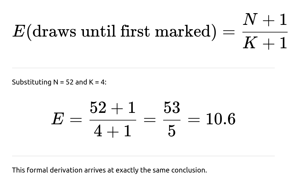
Another way to view this is through the Negative Hypergeometric Distribution, which models the number of draws from a finite population containing a certain number of “marked” elements (aces in this case) until the first marked element appears. If you let:
M = 4 (the number of aces),
N = 52 (the total number of cards),
K = the number of marked cards (again 4 aces), then the expected value of the number of draws until the first ace is:

Connection to Uniform Spacing
The “divider” analogy is closely related to the uniform spacing idea in combinatorics and probability. If you label four aces and think of them as fixed points, the other cards are being randomly permuted around them. In essence, this is the same as having five regions where these 48 non-aces can fall, leading to the same average count in each region.
Practical Considerations
The derivation gives us a mean (expected) number of cards. Actual draws will vary from game to game.
The linearity-of-expectation principle often simplifies calculations that might otherwise be approached through sum-of-probabilities approaches or combinatorial enumeration.
Real-world card draws will yield discrete outcomes; 10.6 is simply the long-run average over many hypothetical deals or simulations.
Potential Follow-up Question: Formal Derivation with Sums
A more classical method involves summing the probabilities that the first ace appears on the k-th draw. This leads to terms involving combinations of how many non-aces precede the ace. Could you show such a derivation?
When we try to compute it directly, we consider:
The probability that the first k–1 cards contain no aces.
Then multiply by the probability that the k-th card is an ace.
One can write a summation for the expected value:
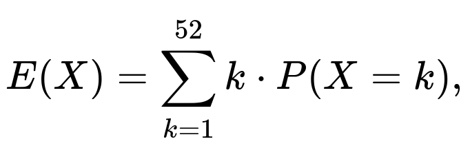
where ( P(X = k) ) is the probability that the first ace occurs exactly on the k-th draw. That probability in turn involves combinatorial coefficients for how many ways to place non-aces in the first k–1 positions and an ace in the k-th, relative to all possible permutations of the deck. This process can be tedious but confirms the result of 10.6.
Potential Follow-up Question: Simulation Approach
How can we confirm this result with a Python simulation?
A simulation can be done by shuffling a deck repeatedly, counting how many cards are drawn until the first ace appears, and then averaging over many trials. Here is a straightforward code example:
import random

def simulate_first_ace_draws(num_simulations=100_0000):
    import statistics

    deck = [i for i in range(52)]  # Let's label cards 0 to 51
    # Suppose indices 0 to 3 represent the 4 aces, and 4..51 represent non-aces

    results = []
    for _ in range(num_simulations):
        random.shuffle(deck)
        count = 0
        for card in deck:
            count += 1
            # If it's one of the 4 aces
            if card < 4:
                results.append(count)
                break

    return statistics.mean(results)

# Run the simulation
avg_draws = simulate_first_ace_draws()
print("Approximate average number of draws until first ace:", avg_draws)
In practice, this simulation result should gravitate toward 10.6 as the number of simulations grows large.

Potential Follow-up Question: Edge Cases and Variations
What if we had a smaller or larger number of special cards? Could the same logic extend?
Yes, the same logic works. If you have ( M ) special (marked) cards in a deck of ( N ) total cards, then thinking of those ( M ) cards as dividers creates ( M+1 ) gaps. You have ( N - M ) non-special cards distributed among these ( M+1 ) gaps, leading to an expected ((N - M)/(M+1)) cards before the first special card, and hence the total including that special card is ((N - M)/(M+1) + 1).
Potential Follow-up Question: Continuous Analogy
Is there a continuous counterpart to this type of problem?
Yes. In continuous probability, there is a concept of "arrival times" in Poisson processes, where the expected waiting time before the first event (or arrival) is the inverse of the rate parameter (\lambda). Although the finite deck problem is discrete and the Poisson process is continuous, the spirit of “waiting time until the first occurrence” is similar in both contexts.
Potential Follow-up Question: Practical Application in Machine Learning
How is this concept relevant in ML or data science?
While this card problem might seem purely recreational, the underlying principles of expected values and “first success” probabilities are vital in areas like:
Stochastic gradient descent convergence analysis (how many iterations until a certain loss threshold is hit).
Queueing theory in system performance (how many arrivals until a system overload).
Bayesian updating (how many trials until evidence for a certain hypothesis is first observed).
Recognizing how to quickly compute expected times until first success is crucial when designing, simulating, or analyzing probabilistic algorithms in data science and machine learning.
Below are additional follow-up questions
How does this expectation change if the deck is incomplete or has extra cards?
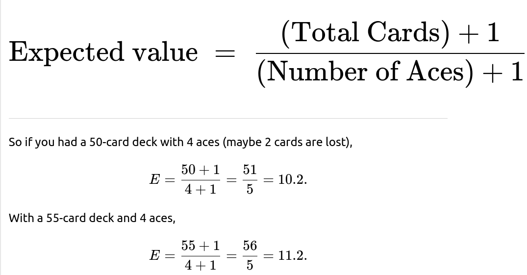
One potential twist is when the deck isn't the standard 52 cards. Suppose some cards are missing or extra promotional cards are included. If, for instance, you only had 50 total cards (with the same 4 aces) or 55 cards (still 4 aces), you might wonder how that affects the expected number of draws.
Detailed Answer
In the general formula using the “divider” principle, the count of non-ace cards changes from 48 to something else, say (n), while the number of aces remains at 4. In that scenario, the 4 aces still define 5 gaps, but now there are (n) non-aces to spread among those 5 segments. The expected number of non-aces before the first ace would thus be (n/5). After including the first ace itself, you get (n/5 + 1).
From a purely algebraic perspective, or using the negative hypergeometric viewpoint, you’d have:
Potential pitfalls and real-world issues
If you don’t know exactly how many cards are missing or how many aces remain, you can only compute an expected value if you have reliable estimates of the deck composition.
In an actual casino or game setting, a miscounted deck might change the odds dramatically, but you’d rarely be aware of it.
Ensuring the deck is thoroughly shuffled remains a separate concern: a partial deck with a poor shuffle can systematically skew the distribution of aces.
Does the expectation depend on how well the deck is shuffled?
Randomness in shuffling is an assumption crucial to most probability calculations for card problems. If the shuffle is imperfect, it might bias the position of certain cards.
Detailed Answer
If we assume a well-shuffled deck, each permutation of the 52 cards is equally likely, and the “divider” argument or negative hypergeometric distribution approach holds exactly. But if the deck is only partially shuffled, there could be “clumps” of cards that remain together. In extreme cases (e.g., a deck that has not been shuffled at all), you might see all four aces near the top or bottom, or locked together in the middle.
Potential pitfalls and real-world issues
In real gaming scenarios, multiple thorough shuffles are used, sometimes with machine shufflers. Even then, some non-uniformities can happen, though they’re generally negligible.
With repeated partial shuffles (like in casual play), certain “tracks” of the deck might remain correlated, invalidating the uniform-permutation assumption.
To apply theoretical results in real life, one usually trusts the deck is near-uniformly shuffled. If you suspect bias, you’d have to model that bias, potentially altering the probability distribution.
What if we only draw from the top half of the deck?
Another variant is: “Imagine you only plan to draw at most 26 cards. On average, how many do you need to draw until you get the first ace?” or “What if you stop if you haven’t found an ace by the 26th draw?” This modifies the scenario because you no longer consider drawing through the entire deck.
Detailed Answer
Stopping after 26 draws: The probability distribution for the first ace changes because there's now a hard limit. You can no longer have the first ace appear on draw 27, 28, etc.
Expected draws: You would calculate a conditional expectation given that you are only drawing from the first 26 cards. Let ( X ) be the random variable for “the draw on which the first ace appears.” You’d look at ( P(X = k \mid X \le 26) ). If the deck is well shuffled, this is akin to looking at the arrangement of the top half of the deck in isolation.
For instance, the chance that the first ace is at position ( k ) among the top 26 can be computed by enumerating or using combinatorial arguments restricted to those top 26 positions. But the bottom line is that your maximum possible ( k ) is 26, which changes the distribution and might reduce the expected number of draws if, for example, more times you end up “not seeing any ace at all” within that range (in which case you might define the variable differently or treat “no ace found” as 27 by default).
Potential pitfalls and real-world issues
If you define “expected draws until the first ace” but have a stopping criterion, you need a convention for what happens if no ace appears by the stopping point. This can shift the analysis to a truncated distribution.
In real card games, sometimes players only look at a subset of their deck. The classical formula assumes you can potentially go through all 52 cards if needed.
How would the expectation change if we look for the second ace instead of the first?
This question generalizes the problem: “After the first ace, how many additional draws (on average) until we see the second ace?” or more simply, “What is the expected number of draws until we see the second ace from the beginning?”
Detailed Answer
For the second ace from the beginning: You can again use the uniform-gap approach, but now you have 4 aces defining 5 gaps, and you are interested in the sum of the first gap plus the first ace plus the second gap plus the second ace. In terms of the negative hypergeometric distribution, you want the expected number of draws until 2 aces have appeared.
The direct formula for the negative hypergeometric approach is more involved for the second, third, or fourth success. However, you could break it down into:
Expected draws to see the first ace.
Then expected additional draws to see the next ace from that point onward.
By linearity of expectation, you can sum these. But you must be mindful that after seeing the first ace, you effectively have a deck of 51 cards with 3 remaining aces. So the expected number of additional draws to see the next ace might be:
But that 51-card deck scenario is not always exactly “shuffle from scratch,” because we know some partial order was already established. If we assume each arrangement was equally likely to begin with, the memoryless property doesn’t hold in a purely combinatorial sense the same way it does in a geometric distribution. Still, on average, you can do a staged approach for the expectation.
Potential pitfalls and real-world issues
The distribution for the second, third, and fourth ace is not as straightforward as for the first ace, because once you start removing cards, the deck has changed.
Some card players incorrectly assume a geometric-like memorylessness if they see “no ace in the first 10 cards,” but that assumption only holds if we re-shuffle or if we had incomplete knowledge. In a well-ordered but unknown deck, partial knowledge does update the probabilities.
How does partial knowledge of card locations impact the expected draw count?
Sometimes, you might know something about the location of an ace. For instance, if you caught a glimpse of a card while shuffling or if some portion of the deck was revealed as having no aces. How does this partial information change the expected number of draws?
Detailed Answer
Any knowledge that modifies the distribution of where the aces could be affects the calculation. For example, if you know the top 5 cards contain no ace, then for the first ace, you have effectively a 47-card deck (with all 4 aces) starting from position 6 onward. Now the expectation becomes:
but that is the expected draw “starting from card 6.” So from the perspective of the entire deck, it might take (5 + 9.6 = 14.6) total draws on average, because you already looked at 5. More nuanced partial knowledge—like “there is at least one ace in the top 10, but not in the top 2”—would need more delicate conditional probability calculations.
Potential pitfalls and real-world issues
In practice, partial knowledge is common, e.g., when a dealer accidentally exposes a card or if a game’s rules involve open “burn” cards.
Failing to update your distribution to incorporate new information leads to incorrect predictions about the likelihood of drawing an ace soon.
Could a dependence structure among cards (beyond just random placement) cause surprising results?
Sometimes, real decks or specialized games have non-standard distributions of cards. If certain suits or ranks clump together or if aces are intentionally placed, we break the assumption of uniform randomness.
Detailed Answer
If the deck is arranged with some dependency—say in a magic trick or cheating scenario—the usual formulas collapse. The expected time to the first ace might be artificially lowered if a “cooler” deck is set up with aces near the top, or raised if an “anti-luck” arrangement is forced. Such manipulations can be invisible if done skillfully.
Potential pitfalls and real-world issues
Relying on the standard 10.6 figure in a rigged setting is unwise because it assumes fair shuffling.
In machine learning contexts, any correlation or dependence in the data that violates i.i.d. assumptions can lead to incorrect model training or inference. Likewise, for card draws, if they aren’t i.i.d. permutations, the fundamental assumption is broken.
What about repeating the experiment multiple times and averaging the results manually?
Someone might physically shuffle a deck many times, draw until they find the first ace, record how many draws it took, and compute the average. They might wonder if they’ll see exactly 10.6 on average or if any random variation could mislead them.
Detailed Answer
Practical repeated trials: If you do, say, 30 trials, your sample average might deviate from 10.6 due to sampling variability. If you do 10,000 trials (either physically or via computer simulation), the sample mean will likely converge near 10.6 due to the Law of Large Numbers.
Confidence intervals: For a finite number of trials (n), the sample mean has a distribution around the true mean. One could estimate standard deviations and construct confidence intervals. The negative hypergeometric distribution can be used to approximate standard deviation, or you can do it empirically from the repeated trials.
Potential pitfalls and real-world issues
In real card draws, it’s cumbersome to do thousands of trials manually. Even a small systematic error in shuffling or data recording can bias the results.
Online or real-casino streams might give data for partial draws only. Missing data or partial draws complicate the analysis.
Can the result be generalized to seeking the first appearance of any specific rank or suit?
Another question is if we’re looking for the first King, or the first spade, or any arbitrary “special” set of cards.
Detailed Answer
The principle applies generally to the negative hypergeometric distribution, which covers “how many draws from a finite population until the first (or k-th) success” in a scenario with known numbers of successes. So if the “special” cards are:
13 spades in a 52-card deck,
4 kings in a 52-card deck,
or 8 black cards (spades + clubs) for a partial scenario,
the formula simply uses (K) as the number of special cards, (N) as the total deck size, and yields:

Potential pitfalls and real-world issues
If the rank or suit is unevenly distributed (deck misprints, missing suits, jokers labeled as wild, etc.), you need to adjust the count of “special” cards accordingly.
Always check your assumptions about how many target cards exist and whether those cards are guaranteed to be there (e.g., no card is lost).
Is there a way to interpret this result in terms of classic “coupon collector” style reasoning?
Some might try to connect “waiting time to first ace” with the well-known coupon collector problem, where you wait until you collect all coupons (or all card ranks).
Detailed Answer
Coupon collector: You have 13 ranks, and you want at least one of each rank. On average, it takes (13 \times H_{13} \approx 13 \times 3.8 ) = 49.4 draws to collect them all, where (H_{13}) is the 13th Harmonic number.
First-ace problem: You only need the first instance of one rank, specifically aces. Rather than collecting them all, you’re satisfied with just one success. So it is more akin to a “first success” problem and not a “collect them all” scenario.
Although these problems both involve drawing from a finite set with replacements or permutations, they differ in what “success” means (the coupon collector problem is about collecting every type, whereas the first-ace problem only needs one success). The coupon collector has a distribution with typically longer waiting times because you need multiple successes spread across different categories.
Potential pitfalls and real-world issues
Conflating the two can lead to incorrect assumptions about how many draws are needed for a single success versus multiple successes.
In interviews, clarifying the difference helps demonstrate a strong conceptual understanding of distinct probability setups.
Could we modify this question to a “first card of a certain color or suit appears” with a known distribution of suits?
If the question is about color (say red vs. black), you have 26 red and 26 black cards. The logic is similar: you’re looking for the first occurrence of one of those 26 red cards.
Detailed Answer
Applying the same negative hypergeometric formula for the number of “red” cards, which is (K=26), the expected position for the first red card is:

Meaning, on average, you only expect to get through about one or two cards before seeing a red card if the deck is well shuffled. This is intuitive because half the deck is red.
Potential pitfalls and real-world issues
A subtle error can arise if the deck is not balanced (e.g., 25 reds and 27 blacks, or if a card is missing).
Mislabeling suits or ignoring that the deck might be stacked can cause big differences in the expected count.
What if we draw cards with replacement instead of without replacement?
A question might arise if each draw is replaced back into the deck (and the deck reshuffled). That changes the distribution from a hypergeometric to a geometric or negative binomial setup.
Detailed Answer
With replacement: Each draw is an independent Bernoulli trial with probability (p = \frac{4}{52} = \frac{1}{13}) of drawing an ace. The expected number of draws until the first success in a geometric distribution is (1/p = 13). That’s different from 10.6 because, with replacement, the probability of drawing an ace remains constant over draws.
Without replacement: That’s our original scenario. Each draw changes the composition of the deck and modifies the probability of drawing an ace on subsequent draws.
Potential pitfalls and real-world issues
Confusing these two scenarios is a common mistake in probability interviews.
Always confirm whether draws are made with or without replacement. In real card games, it’s typically without replacement, but in some sampling settings (like certain sampling algorithms in data science), it may be with replacement or partially so.
Could counting aces in someone’s hand be affected by the order the cards are dealt?
In typical card games, players receive hands of 5 (or more) cards in some order. Does the order matter, or is it effectively the same as random draw?
Detailed Answer
If you are only looking at your personal 5-card hand (and ignoring others), the order in which the 5 cards are handed to you doesn’t matter for how many aces you end up with. However, if you specifically ask, “Which position in my 5-card hand is typically the first ace I see?” then the order does matter. The distribution might look different if you consider that the dealer deals “round-robin” to multiple players.
In a typical 5-card deal from a well-shuffled deck, each subset of 5 cards is equally likely. The position within that 5-card hand is uniformly random, but only among the 5 cards you receive, not among the entire deck.
If multiple players are being dealt cards, your draws are interspersed with theirs, which can complicate the direct interpretation of the “first ace drawn.” Yet from a purely random permutation perspective, it’s still ultimately random which card arrives to you in which position.
Potential pitfalls and real-world issues
Overthinking the dealing order can confuse the simpler fact that each 5-card hand is equally likely.
If you specifically track the first ace across multiple players, you need to incorporate the possibility that an ace arrives to someone else first (which is a different question).
What if the four “aces” are not identical? Could the result differ if we care which ace we see first?
Some might wonder if labeling the aces distinctly (A♠, A♥, A♣, A♦) changes the expectation. For example, “What is the expected position of the Ace of Spades specifically?”
Detailed Answer
The expected position for the first of the four aces (treated as an undifferentiated event “seeing any ace”) is 10.6.
However, if you specifically want the Ace of Spades alone, that’s a single card among 52. The expected position of a single specified card in a randomly shuffled deck is (\frac{52+1}{2} = 26.5). That’s because, for one special card, there are 2 “gaps” (before and after it), so you get ( \frac{52 - 1}{2} = 25.5 ) other cards on average before it, plus 1 for the card itself. More straightforwardly, a single card is equally likely to be anywhere among 52 positions. So its average position is ((1 + 52)/2 = 26.5.)
If you want the first time you see a specific labeled ace out of the four total distinct aces, you must be careful about “which event triggers the stop.” That’s a different question than “first ace” if not all aces are considered the same.
Potential pitfalls and real-world issues
Confusing “seeing any ace” with “seeing a specific ace” can cause mix-ups in expected positions.
In many games, suits and ranks might have different significance, so the “first ace” question might not match “first Ace of Spades” question. They yield different results.
Does the shape of the probability distribution matter, or do we only care about the mean?
Sometimes an interviewer wants to see if you understand variance and higher-order moments. “Yes, the expected value is 10.6, but how spread out is the distribution?”
Detailed Answer
For the negative hypergeometric distribution describing “first success,” the variance can be derived from its standard formula. While 10.6 is the average, the distribution can allow for quite early appearances (e.g., 1 or 2) or quite late appearances (all the way near the 49th or 50th card).
The variance for the negative hypergeometric with parameters ((N, K)) for the first success is more involved, but can be computed using known closed-form expressions or a direct combinatorial approach.
Understanding this helps to gauge “risk” or “uncertainty.” Even though the mean is 10.6, you can get the first ace on the very first draw or not until extremely late in the deck.
Potential pitfalls and real-world issues
Over-reliance on the mean might cause you to underestimate the likelihood of extremes.
In real card-based strategies, you might want to consider not just the average but also how frequently a particular event might happen in the first few draws, which is directly tied to the distribution’s shape.
Is there a limit to applying the "divider" argument if we had a large number of target cards?
Sometimes, interviewers try to see if the logic still holds if we have many “marked” cards. If you had, say, 26 marked cards, do we still consider them as dividers?
Detailed Answer
Yes, the concept generalizes. If we have (K) marked cards, we have (K+1) gaps among them. For “finding the first marked card,” the expected count of unmarked cards in the first gap is (\frac{N-K}{K+1}). Then you add 1 for the marked card itself. The formula:

So whether (K=4) or (K=26), the principle is the same. The “divider” argument remains valid as long as we treat all permutations of the deck as equally likely.
Potential pitfalls and real-world issues
For a large fraction of marked cards, the average waiting time can be relatively short. For instance, if half the deck is “marked,” the expected number of draws to the first one is roughly 2.
If (K) is so large that almost every card is “marked,” the question becomes somewhat moot, but mathematically it still holds.
Does the “linearity of expectation” help even when events are dependent?
Interviewers sometimes ask you to clarify that linearity of expectation holds even with dependencies. How does that apply here?
Detailed Answer
Linearity of expectation always holds, no matter if random variables are dependent or independent. In the “divider” method, the reasoning about equal distribution of non-aces among the 5 gaps does not explicitly rely on independence in the usual sense; it uses the symmetry of all permutations.
The straightforward approach: Let (X) be the number of draws until the first ace. You can express (X) as (\sum_{i=1}^{52} I_i), where (I_i) is an indicator random variable that says “Do I get to draw the i-th card?” or “Does the process continue at least until card i?” The logic can be broken down, but overall, we rely on symmetrical arguments or direct negative hypergeometric reasoning.
Potential pitfalls and real-world issues
Some confuse linearity of expectation with the requirement of independence. But expectation is additive regardless.
Misunderstanding or mixing up independence can lead to incorrectly applying or dismissing powerful expectation-based shortcuts.
What if the first ace is found, but we continue drawing to see if the second ace appears soon afterward? How does that interplay with the expected count to the first ace?
This question addresses situations where the draws don’t stop after the first ace. You still might be interested in how soon the second ace shows up relative to the first.
Detailed Answer
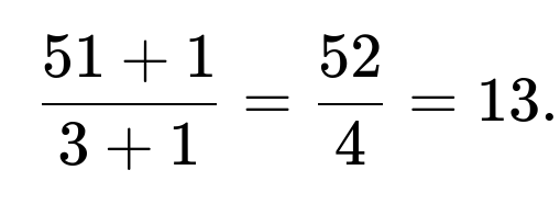
The expected position of the first ace is 10.6. If you keep drawing, you can similarly compute the distribution for the position of the second ace from the deck’s start or from the event of the first ace. The latter is more complicated because, once the first ace is drawn, you’re no longer sampling from the full 52 cards but from the remainder that’s left.
However, by the time you see the first ace, you have an updated situation: there are 51 cards left, 3 of which are aces. If you now treat that as a new problem with 51 total and 3 “marked,” you could say the expected additional draws to see the next ace is (\frac{51 + 1}{3 + 1} = 13). This is a high-level approach ignoring the “position knowledge” from how many non-aces have already appeared, but on average it aligns well with the negative hypergeometric logic.
Potential pitfalls and real-world issues
If you precisely track how many of the first 10 or 11 cards were aces or non-aces, that knowledge refines your distribution. The above reasoning is a rough conditional approach.
Real card game decisions sometimes hinge on partial knowledge. For example, in some strategy card games, if you’ve seen how many key cards have already passed, you change your playing strategy accordingly.
Could this result have real-life parallels in data sampling scenarios, like anomaly detection?
Interviewers may try to see if you can translate the logic beyond card games: “In anomaly detection, how many samples do we typically examine before we find our first anomaly?”
Detailed Answer
In many real-life sampling processes, you look for the first occurrence of an “unusual” event (analogous to an ace). If your data set has a known fraction of anomalies (similar to the fraction of aces in a deck), you can adapt the negative hypergeometric or geometric approach depending on whether you’re sampling from a finite pool (without replacement) or an infinite stream (with replacement).
The expected time until the first anomaly appears is crucial for designing alert systems or real-time monitors.
Potential pitfalls and real-world issues
Real anomalies might not be perfectly and uniformly distributed, unlike well-shuffled cards. They might cluster or show patterns over time.
If the fraction of anomalies is only estimated (and not exact), the theoretical expectation is an approximation. In practice, you calibrate your detectors and might see significantly different results.
What’s a common misconception learners might have about this result?
Understanding 10.6 can be counterintuitive to many who initially guess something around 13 (since 1/13 chance for any given draw in a with-replacement sense).
Detailed Answer
A frequent misconception is to conflate the deck-without-replacement scenario with a simpler Bernoulli process. In the with-replacement scenario (geometric distribution), you expect 13 draws for the first ace. But with no replacement, it’s slightly less because each non-ace drawn actually improves the chance that the next card is an ace.
Potential pitfalls and real-world issues
Failing to distinguish between these two sampling models leads to confusion about why 10.6 is smaller than 13.
In an interview, clarifying “without replacement” is key to showing you understand the subtle but important difference between hypergeometric and geometric sampling.