
ML Interview Q Series: Expected Heads for Conditional Coin Tosses Solved via Difference Equations.

Browse all the Probability Interview Questions here.
You have two coins. One coin is fair and the other is biased with probability p of heads. The first toss is done with the fair coin. At the subsequent tosses, the fair coin is used if the previous toss resulted in heads, and the biased coin is used otherwise. What is the expected value of the number of heads in r tosses for r = 1, 2, … ?
Short Compact solution
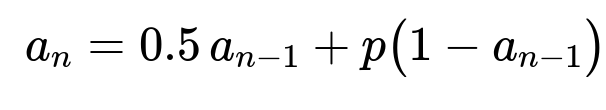
Let I_n be the indicator variable that is 1 if the nth toss results in heads and 0 otherwise. Define a_n = P(I_n = 1). By conditioning on whether the previous toss was heads or tails, we obtain the difference equation:

Comprehensive Explanation
Overview of the Problem Setup
We have two coins:
A fair coin (probability of heads = 0.5).
A biased coin (probability of heads = p).
The procedure for tossing coins is:
The very first toss (n = 1) is always done with the fair coin.
For each subsequent toss (n ≥ 2), we observe the result of the previous toss:
If the previous toss was heads, we toss the fair coin next.
If the previous toss was tails, we toss the biased coin next.
We want to compute the expected total number of heads over r tosses.
Defining the Indicator and Recurrence
Let I_n = 1 if the nth toss is heads, and I_n = 0 otherwise. Then the expected number of heads in r tosses is the sum of the expected values of these indicators:
E[∑ from n=1 to r of I_n] = ∑ from n=1 to r of E[I_n].
Define a_n = P(I_n = 1). Notice that E[I_n] = a_n because the expectation of a Bernoulli random variable is just its probability of being 1. Hence, we only need to find each a_n and sum them.
To find a_n, we apply conditional probability based on the previous outcome:
a_n = P(I_n = 1) = P(I_n = 1 | I_{n-1} = 1) * P(I_{n-1} = 1) + P(I_n = 1 | I_{n-1} = 0) * P(I_{n-1} = 0).
From the problem statement:
If I_{n-1} = 1 (previous toss was heads), then the nth toss uses the fair coin with probability of heads = 0.5.
If I_{n-1} = 0 (previous toss was tails), then the nth toss uses the biased coin with probability of heads = p.
Hence, P(I_n = 1 | I_{n-1} = 1) = 0.5, P(I_n = 1 | I_{n-1} = 0) = p,
and P(I_{n-1} = 1) = a_{n-1}, P(I_{n-1} = 0) = 1 − a_{n-1}.
Therefore,

Solving the Difference Equation
We have a first-order linear difference equation of the form:
a_n = (constant) * a_{n-1} + (constant).
Rewriting:
a_n = (0.5 − p) a_{n-1} + p.
However, it is typical to keep it in the original form:
a_n = 0.5 a_{n-1} + p (1 − a_{n-1}).
We also have an initial condition for a_1. Since the first toss is with the fair coin, a_1 = 0.5.
A standard method to solve such equations is either by iteration or by recognizing it as a linear recurrence:
a_n − 0.5 a_{n-1} − p(1 − a_{n-1}) = 0, a_n − (0.5 + p) a_{n-1} + p = 0.
Solving in a closed form, we get:

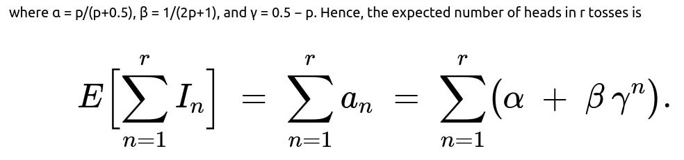
where one typically determines α by finding the steady-state solution (when a_n = a_{n-1} = a, so a = 0.5 a + p(1 − a)) and β, γ by plugging back into the difference equation and using the initial condition a_1 = 0.5. From the snippet we have:
α = p / (p + 0.5).
β = 1 / (2p + 1).
γ = 0.5 − p.
Expected Value Calculation
Because E[I_n] = a_n, the expected total number of heads over r tosses is:

One can evaluate this sum explicitly, if desired, using the formula for the sum of a geometric series for the βγ^n part. In many practical interview solutions, leaving the final expression as ∑(α + β γ^n) for n=1..r is already acceptable.
Practical Simulation (Optional)
In practice, one might simulate this process for large r to verify the derived formula matches the empirical average. A simple Python example:
import numpy as np

def simulate_expected_heads(p, r, trials=10_000_00):
    # p: biased coin probability
    # r: number of tosses
    # trials: number of Monte Carlo trials
    counts = []
    for _ in range(trials):
        coin_result = np.zeros(r)
        # First toss: fair coin
        coin_result[0] = 1 if np.random.random() < 0.5 else 0
        for i in range(1, r):
            if coin_result[i-1] == 1:
                # Use fair coin
                coin_result[i] = 1 if np.random.random() < 0.5 else 0
            else:
                # Use biased coin
                coin_result[i] = 1 if np.random.random() < p else 0
        counts.append(np.sum(coin_result))
    return np.mean(counts)

# Example usage:
p = 0.7
r = 10
est = simulate_expected_heads(p, r)
print("Monte Carlo estimate of expected heads:", est)
This simulation provides a rough numerical check of the derived closed-form expression.
Potential Follow-up Question 1
How do we interpret the steady-state behavior of the sequence a_n for large n?
When n grows large, the term β (γ^n) goes to 0 if |γ| < 1. Here, γ = 0.5 − p.
If 0 < p < 0.5, then |0.5 − p| < 1, so a_n converges to α = p / (p + 0.5).
If p ≥ 0.5, then |0.5 − p| ≤ 0, leading to a different boundary behavior (for example, if p = 0.5 exactly, then γ = 0, and a_n stabilizes even more quickly).
Hence, in the long run, the probability of getting heads on any given toss stabilizes at α.
Potential Follow-up Question 2
What if p = 0.5? Does that make both coins fair? How does it affect the formula?
If p = 0.5, both coins are fair coins. From the recurrence relation, a_n = 0.5 a_{n-1} + 0.5 (1 − a_{n-1}) = 0.5, regardless of a_{n-1}.
The solution trivially becomes a_n = 0.5 for all n.
Therefore, the expected number of heads in r tosses is 0.5 * r.
Potential Follow-up Question 3
What if p = 1 or p = 0?
If p = 1, the biased coin always lands heads. Then whenever you get tails (which is impossible if you keep tossing the biased coin—since it can’t give tails if p=1), you'd keep using the biased coin. Actually, more concretely:
The first toss is fair. If it’s heads, you keep using the fair coin (0.5 chance). If it’s tails (0.5 chance), you switch to the “biased” coin that is always heads.
From that point on, once you ever toss tails with the fair coin, you move to the always-heads coin and stay there. So you can see a dramatically increased number of heads over time.
If p = 0, that means the biased coin always lands tails. You only stay with the fair coin if it results in a head. If ever the fair coin yields tails, you switch to a coin that can never produce heads. Over a large number of tosses, you very quickly end up stuck with no heads once you switch to the p=0 coin.
These extremes illustrate the importance of the difference equation approach, because it naturally accounts for switching behaviors based on previous outcomes.
Below are additional follow-up questions
What if we are also interested in the variance of the total number of heads over r tosses, not just the expected value?
One way to approach this is to write the total number of heads as the sum of the indicator variables I_n for n=1 to r and then use Var(∑ I_n) = ∑ Var(I_n) + 2∑ Cov(I_m, I_n) for m<n. The main challenge is figuring out P(I_m=1, I_n=1) for m<n, which depends on the Markovian coin-switching mechanism. The chain of dependencies can be captured by enumerating states or by direct calculations using conditional probabilities.
A subtle pitfall is failing to account for correlations between tosses. Unlike a sequence of i.i.d. Bernoulli random variables, here each toss’s success probability a_n depends on the previous outcome. Attempting to do Var(∑ I_n) = ∑ Var(I_n) alone would ignore the covariance terms, which can lead to incorrect results. In real-world interviews, an improper assumption of independence is a common mistake.
Could we frame this coin-switching process as a Markov chain and leverage that framework?
Yes. We can define a Markov chain with two states: “Heads on the previous toss” and “Tails on the previous toss.” The transition probabilities reflect which coin is used next:
From “Heads on previous toss” to “Heads on current toss,” the probability is 0.5.
From “Heads on previous toss” to “Tails on current toss,” the probability is 0.5.
From “Tails on previous toss” to “Heads on current toss,” the probability is p.
From “Tails on previous toss” to “Tails on current toss,” the probability is 1 − p.
Each toss’s outcome is then a direct sample from the state-based coin. This viewpoint makes it easier to see the steady-state behavior: once the chain reaches equilibrium, the chance of being in each state stabilizes. A common pitfall is to assume states revolve around “which coin is used,” while ignoring that the usage depends strictly on the previous result. In interviews, discussing Markov chains can demonstrate a candidate’s deeper grasp of stochastic processes.
What happens if the first toss was accidentally done with the biased coin instead of the fair coin?
This changes the initial condition of our difference equation. Instead of having a_1 = 0.5, we would have a_1 = p. For subsequent tosses, the same recurrence a_n = 0.5 a_{n-1} + p(1 − a_{n-1}) still applies. Hence the primary difference is that the solution’s constants (for example, the coefficient β in the term βγ^n) would adjust to accommodate the new a_1.
A subtlety is that the overall limit behavior for large r won’t change; the sequence still converges to the same steady-state probability α = p / (p + 0.5). The difference is in how quickly or slowly it approaches that steady-state and how the total count of heads accumulates. In real implementations or when verifying results, confusion can arise if one forgets to adjust that initial condition, leading to incorrect short-run estimates.
How can we generalize if we had multiple coins with different probabilities, and the choice of which coin to use depends on more complicated rules?
We can still set up a Markov chain with states reflecting whatever information is needed to decide which coin is used next. For instance, if the rule is that the next coin depends on the last two outcomes, we would track states based on that 2-step history. The dimension of the chain grows with the complexity of the rule, but the principle is similar.
A pitfall is that as the rule grows more complex (such as depending on multiple previous outcomes), the state space can explode combinatorially. In an interview, one might emphasize how to handle the resulting complexity or approximate it (e.g., with a simulation if an analytic solution becomes unwieldy).
If we wanted the probability distribution of the total number of heads instead of just its expectation, how might we proceed?
We could iterate over all sequences of heads/tails up to length r, tracking probabilities of each sequence. More efficiently, a dynamic programming approach can be used: we keep track of the probability that exactly k heads occur after n tosses while noting which coin is used for the nth toss. This also effectively becomes a Markov chain approach in higher dimensions, where we track (number of heads so far, state of previous toss).
A common pitfall is underestimating how quickly the number of possible sequences grows (2^r in the worst case). For large r, direct enumeration is impractical, so either dynamic programming or an approximation technique is needed. In real-world contexts, approximate methods (e.g., Monte Carlo) often strike a balance between complexity and accuracy.
How sensitive is the expected number of heads to small changes in p?
From the closed-form solution a_n = α + β γ^n, where γ = 0.5 − p, even tiny deviations in p can affect γ significantly if p is near 0.5. When p is close to 0.5, a small change can push γ from slightly negative to slightly positive or vice versa, influencing the speed at which a_n approaches α. In turn, the total expected number of heads could shift measurably over r tosses for moderate r.
A real-world pitfall is ignoring that near p = 0.5, you may see an amplified effect on short-run behavior. Interviewers might ask you how you’d validate or stress-test a real system to ensure the estimates remain robust to parameter drift (e.g., hardware coin tosses that aren’t perfectly unbiased, or data collection noise that misestimates p).
What if the parameter p itself is unknown, and we need to estimate it on the fly while tossing coins?
In such scenarios, we have a partially observable process: we do not know p exactly but keep gathering heads/tails data from a mixture of the fair coin and the biased coin. One approach is to treat p as a parameter and use a Bayesian update or maximum likelihood approach while recognizing that each observed toss is not an i.i.d. sample from the same Bernoulli distribution but a sample from a “coin-switching” mixture. We might use an Expectation-Maximization (EM) procedure or a Markov chain model with an unknown transition probability we continuously learn.
A subtlety is that naive estimation might assume a single Bernoulli distribution for all tosses and thereby produce a heavily biased estimate. Correctly separating which tosses came from the fair coin vs. the biased coin can be nontrivial because the usage depends on previous outcomes. In an interview, discussing how to adapt standard parameter estimation to account for a piecewise coin usage pattern often showcases advanced understanding.