ML Interview Q Series: Expected Married Couples in Random Teams using Linearity of Expectation.

Browse all the Probability Interview Questions here.

Question: Twelve married couples participate in a tournament. The group of 24 people is randomly split into eight teams of three people each, where all possible splits are equally likely. What is the expected value of the number of teams with a married couple?

Short Compact solution

Let I_k be an indicator variable that is 1 if the k-th team has at least one married couple, and 0 otherwise. The probability that any given 3-person team has a married couple is 12 * 22 / (24 choose 3). By linearity of expectation, the expected number of teams that contain at least one married couple is 8 * 12 * 22 / (24 choose 3), which numerically evaluates to approximately 1.043.

Comprehensive Explanation

Using Indicator Variables and Linearity of Expectation

A clear way to tackle this problem is through indicator random variables:

• We label each team k = 1, 2, …, 8.

• Define I_k = 1 if team k contains at least one married couple, and 0 otherwise.

The total number of teams that have a married couple is X = I_1 + I_2 + … + I_8. Our goal is E(X).

According to the linearity of expectation, we have: X = sum_{k=1 to 8} I_k

so E(X) = sum_{k=1 to 8} E(I_k).

Hence, all we need is E(I_k) for a typical team k, and then we multiply by 8.

Computing E(I_k)

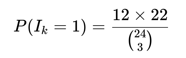
I_k is 1 exactly when the team of three people contains a married couple. The probability that I_k = 1 is:

Explanation of each component:

• The total number of ways to choose any 3 people out of 24 is (24 choose 3).

• To count the number of favorable 3-person groups that contain at least one married couple, we pick which of the 12 couples is included (12 ways). For each chosen couple, we include those exact 2 individuals and then choose 1 more person out of the remaining 22 people. Hence, there are 12 * 22 favorable choices in total.

• Because a 3-person subset cannot contain two distinct couples (that would require 4 people), we do not double-count.

Thus:

E(I_k) = 12 * 22 / (24 choose 3).

Putting It All Together

Since each of the 8 teams has the same probability of including a married couple, we write:

When you compute (24 choose 3) = 2024, the numerical value becomes:

8 * (12 * 22 / 2024) ≈ 1.043.

Therefore, the expected number of teams that contain at least one married couple is approximately 1.043.

Sanity Check via Simulation

Below is a quick Python example to confirm this result empirically:

import math, random
import statistics

def simulate(num_simulations=10_000_00):
    counts = []
    for _ in range(num_simulations):
        # Create list of 24 distinct individuals, grouped in couples
        # We'll label them as pairs: (0,0), (0,1) for couple 0, (1,0), (1,1) for couple 1, etc.
        individuals = [(i, j) for i in range(12) for j in range(2)]
        random.shuffle(individuals)

        # Split into 8 teams of 3
        teams = [individuals[i*3:(i+1)*3] for i in range(8)]

        # Count how many teams have a married couple
        count = 0
        for team in teams:
            # Check if any two are from the same couple
            couples_in_team = set([p[0] for p in team])  # p[0] is the couple ID
            if len(couples_in_team) < 3:  # means at least two from same couple
                count += 1
        counts.append(count)

    return statistics.mean(counts)

sim_estimate = simulate()
print(f"Simulation estimate of expected number of teams with a married couple: {sim_estimate}")

Running a simulation with a sufficiently large number of trials should produce a result close to 1.043.

Follow-Up Question: How do we approach finding the variance of the number of teams that contain a married couple?

To find the variance, you would need Var(X) = E(X^2) - [E(X)]^2. While E(X) is straightforward by linearity, E(X^2) requires knowing E(I_k I_m) for k ≠ m, which depends on the joint probability that both team k and team m contain a married couple. That in turn depends on whether these teams share one or more individuals. You must carefully enumerate cases where team k and team m overlap by 0, 1, or 2 individuals. Each scenario contributes differently to the joint probability.

Follow-Up Question: What if teams had more than three members, say groups of four or five? How would the approach change?

The core strategy would remain similar:

1. Use an indicator variable I_k for each team.

2. Compute P(I_k = 1) under the new group size, because the probability that a randomly chosen group of size g has a married couple will differ.

3. Apply linearity of expectation and sum over all teams.

The main difference is in the combinatorial details: for a group of size g, you count how many ways to choose a married couple (12 ways) and then choose the remaining g-2 individuals from the remaining 24-2 = 22 individuals. You then divide by the total ways of choosing g people out of 24.

Follow-Up Question: If we needed the probability that exactly one team contains a married couple (or exactly k teams), how would we proceed?

In that scenario, simply knowing E(X) by linearity of expectation is not enough. You would need to consider the distribution of X:

• One possible route is to use inclusion-exclusion or advanced combinatorial arguments to handle the probability of exactly k teams containing a married couple.

• Alternatively, you might try a more direct counting approach: first pick which k teams contain couples, ensure each of those k teams has at least one couple, ensure the other teams do not, and account for any overlap constraints. This quickly becomes nontrivial because the ways teams can overlap in members is intricate.

Follow-Up Question: Why is it valid to multiply by 8 after finding E(I_k) if the teams might overlap in some combinatorial sense?

This is precisely where the linearity of expectation is powerful: it does not require the indicators I_k to be independent. Even though the composition of team k might affect the composition of team m, the expected value of their sum is still the sum of their expected values. This is a common technique in probability theory to simplify calculations without worrying about dependencies among events.

All these follow-up topics underscore the flexibility of indicator-variable methods. Despite complicated dependencies in how teams are formed, the linearity of expectation remains an extremely useful tool.

Below are additional follow-up questions

What if the random assignment is done sequentially instead of choosing all eight teams at once?

Even though the typical combinatorial analysis assumes all 24 people are split into teams in a single uniform random draw, in practice, teams might be picked sequentially. For instance, we might choose a random set of 3 people for Team 1, then choose a random set of 3 people for Team 2 out of the remaining 21, and so on.

Detailed Explanation

• Equivalence of Sequential vs. All-at-Once In principle, if each person has an equal chance of landing in any particular team, sequential selection should still sample from the same uniform distribution over all possible partitions. The probability distribution of final team configurations remains the same as it would be in one big random partition.

• Potential Pitfall Confusion can arise if the process imposes restrictions (e.g., if a previously formed team is rejected and re-chosen) or if the selection for later teams somehow depends on earlier team compositions. Such dependencies can cause the assignment to deviate from the uniform distribution over all partitions.

• Why It Matters In many real scenarios, “sequential picks” could inadvertently bias the team composition—for example, if someone tries to prevent certain people from joining or tries to “balance skill levels.” If any non-random constraint is introduced, the probability that couples end up together would no longer match the simple combinatorial ratio.

Hence, if the sequential process is truly random with no biases, our calculation of the expected value still holds. Otherwise, one must revise the probability assumptions to reflect any constraints or non-uniform selection rules.

Could more than one married couple end up on the same 3-person team, and how would that affect the calculation?

In this scenario, each team has exactly 3 people, so it is impossible for two distinct married couples (i.e., four unique individuals) to reside in the same 3-person team. Thus, any 3-person team can contain at most one married couple.

Detailed Explanation

• Impossible Overlap For two couples to be together, you would need 4 individuals. Since each team is limited to exactly 3, it cannot hold two married couples.

• Edge Case With Larger Teams If the team size were, say, 4 or 5, then multiple couples could in principle appear on the same team. That would require more intricate combinatorial counts (because you can have 2 or even 3 couples in the same group, depending on the team size). But for 3-person teams, the overlap of two different couples is simply not possible.

• Effect on Probability Since each team can either have zero couples or exactly one couple, the probability that a team has at least one couple simplifies to the probability that it has exactly one couple. This is why the probability for I_k = 1 can be directly computed as (12 possible couples) * (22 ways to choose a third person) / (24 choose 3).

What are the minimum and maximum possible numbers of teams containing couples, and can these extremes occur?

We know the expected value is about 1.043, but the random variable X (the number of teams that contain at least one married couple) can theoretically take values from 0 up to some maximum. Understanding the range of X can help interviewers see if a candidate grasps edge cases.

Detailed Explanation

• Minimum Possible Value (X = 0) This would mean no team contains a married couple. While unlikely, it is not impossible. It requires that all 24 people are arranged in such a way that no two spouses end up together. For example, you could distribute the 24 individuals in a “perfectly separated” fashion.

• Maximum Possible Value The largest X arises when every one of the 8 teams has a couple. However, we only have 12 couples total. Since each team with a couple “uses up” exactly 2 spouses from that couple, we need 8 distinct couples to fill 8 teams with a married pair each. This is indeed possible, because we have 12 couples—enough to allocate 8 distinct couples to the 8 teams. Thus, the maximum X is 8.

• Real-World Subtleties In practice, if couples sign up as pairs or if they request to be placed on different teams, the actual randomization mechanism might be influenced. The theoretical extremes (0 or 8) assume purely random assignment.

Could a Poisson approximation or any other limiting distribution be used for large numbers of couples?

When the number of individuals and couples becomes very large, sometimes a Poisson approximation can simplify computations of how many teams end up with at least one couple.

Detailed Explanation

• When Poisson Approximation Is Useful A Poisson approximation often applies when events (e.g., the event that a specific team has a couple) are relatively rare and (approximately) independent. For a very large pool of people, each team might have a small probability of containing a couple. If the number of teams is large, the count of teams with couples might be approximated by a Poisson random variable with parameter λ = (number of teams) * (probability a specific team has a couple).

• Why Independence Might Fail In our exact scenario, the events “Team k contains a couple” and “Team m contains a couple” are not independent because the teams draw from the same pool of 24 people. For large numbers of couples and teams, the overlap is less significant, so a Poisson approximation can become more accurate. But for small or modest sizes, correlation might be too strong for the approximation to be truly precise.

• Implications If a company had thousands of participants forming hundreds of teams, we could look at using a Poisson(λ) model to estimate the distribution of the number of teams containing couples. This could guide quick estimates without computing intricate probabilities exactly.

What if some couples are more “likely” to end up on the same team (e.g., by preference or external constraints)?

Our derivation assumes every possible 3-person split is equally likely. In real life, couples might request to be placed together or, conversely, to be separated. If the probability is no longer uniform, the entire approach needs adjustment.

Detailed Explanation

• Non-Uniform Team Assignments If certain couples are favored to be together, we must assign a higher weight to configurations in which they appear in the same team. Conversely, if organizers avoid placing spouses together, such configurations would be underweighted relative to the uniform random scenario.

• Revising the Probability Under a biased assignment, the probability P(I_k = 1) for a typical team k would not simply be 12 * 22 / (24 choose 3). Instead, we would need to account for how the biased algorithm or preferences shift the odds of that couple being selected.

• Practical Computation One might resort to either:

  1. Direct simulation under the new rules.

  2. A custom combinatorial analysis factoring in the constraints or weighting scheme. Both approaches can quickly become much more complicated than the uniform random approach.

How would we derive the entire probability distribution of X (not just its expectation) using direct combinatorial methods?

Sometimes we want not just E(X), but P(X = 0), P(X = 1), P(X = 2), etc. That distribution is much harder to obtain via direct combinatorial counting than using the linearity of expectation.

Detailed Explanation

• Naive Counting We could, in theory, count how many ways to choose 8 teams of 3 such that exactly k of those teams each contain a married couple. This counting quickly explodes in complexity. We must ensure:

  1. We pick which k teams out of 8 each have exactly one couple.

  2. We choose which couples are in those k teams (ensuring no overlap in couples, because a single couple can’t appear in multiple teams).

  3. We choose the specific additional team members who fill out each 3-person squad for those teams with couples.

  4. We choose the teams for the remaining 8-k that contain no couples.

  5. We ensure no duplication of individuals or teams across any selection step.

• Inclusion-Exclusion A more systematic way might be to apply inclusion-exclusion for each of the 12 couples. You would count the number of ways no couples appear, then subtract ways in which at least one couple appears, add back ways in which at least two couples appear, and so on. This is still quite involved.

• Practical Approach In many interview or exam contexts, exact distribution questions are often addressed with advanced combinatorial or generating function techniques, or more simply with a Monte Carlo simulation. The linearity-of-expectation approach remains a neat shortcut for E(X), but it does not provide the distribution.

How might real-world constraints, like skill balancing or position balancing, alter the expected number of teams with couples?

In tournaments, organizers often try to balance teams for fairness—for instance by distributing strong/weak players or mixing novices and experts. Such constraints might collide with the pure randomness assumption used in our derivation.

Detailed Explanation

• Skill-Based Constraints If each team must have a fixed average skill or a mix of skill levels, the process of assigning individuals is no longer uniform among all possible 3-person teams. Certain couples who both have high (or low) skill might be split up to avoid “stacking” one team.

• Gender or Position Balancing Sometimes tournaments require each team to have at least one female and one male player. While that alone might not eliminate the possibility of couples being on the same team, it can reduce or increase the probability depending on how the participants’ gender distribution is accounted for.

• Resulting Impact These sorts of constraints can shift the probability that a team includes a couple up or down compared to the uniform random scenario. Precisely quantifying the effect may require a custom combinatorial or simulation-based approach.