
ML Interview Q Series: Expected Swaps in Random Permutations Equals 0.5: Proved by Linearity of Expectation
Browse all the Probability Interview Questions here.
25. You have n integers 1...n and take a random permutation. For any integers i, j let a "swap" be defined as when i is in j-th position and j is in i-th position. What is the expected value of the total number of such swaps?
This problem was asked by Robinhood (Medium).
Understanding the Problem and Core Reasoning
A key point is that, in a random permutation of the numbers 1 through n, we are looking for pairs (i, j) such that:
The element i is positioned at index j.
The element j is positioned at index i.
We call each such occurrence a "swap." Notice that in a permutation, the index and the element can be viewed as two distinct dimensions: the element is the "value," and its index is the position in the permutation array. A "swap" is effectively a special 2-cycle in the permutation’s cycle decomposition. Concretely, for a pair (i, j), i ≠ j, we want exactly i → j and j → i.
The random permutation means each of the n! permutations is equally likely. We want the expected (average) number of such "swaps" when we consider all possible permutations.
Indicator Random Variables
One of the most straightforward ways to compute an expected value in such combinatorial settings is to use indicator random variables. Define the indicator variable:
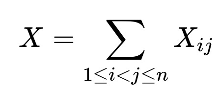
Let X be the total number of (i, j) swaps in the permutation.
For each pair (i, j), with i < j, define an indicator variable X₍ᵢⱼ₎, which equals 1 if the pair (i, j) forms a "swap" and 0 otherwise.
Hence,
Probability That a Specific Pair (i, j) is a Swap
We now calculate the probability that X₍ᵢⱼ₎ = 1 for a particular pair (i, j). This corresponds to the event:
i is in position j.
j is in position i.
Given that each permutation of the n elements is equally likely, we can count the permutations that place i in position j and j in position i. If these two positions are fixed:
There are (n - 2)! ways to arrange the remaining (n - 2) elements.
Therefore, the number of permutations that satisfy this condition is (n - 2)!.
The total number of permutations is n!.
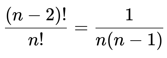
Thus, for a specific pair (i, j), the probability that X₍ᵢⱼ₎ = 1 is:
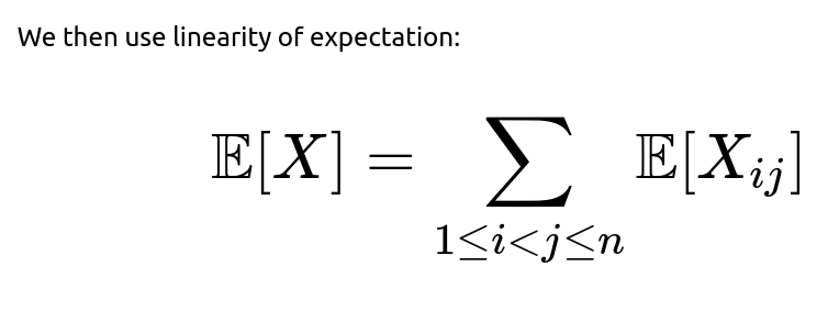
Expected Value Summation
We have n(n - 1)/2 distinct pairs (i, j) when i < j. Summing up:
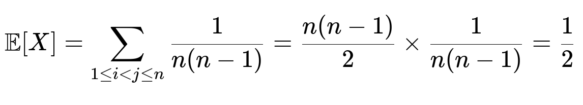
Hence, the expected number of such swaps in any random permutation of the numbers 1 through n is 0.5. This result is quite elegant and perhaps surprising at first, but it aligns with known properties of random permutations and their cycle structures. Intuitively, the existence of any 2-cycle has a relatively small but consistent probability, and averaging across all permutations yields a constant expected value.
Practical Example and Verification by Simulation
To get an intuitive feel for why the expected number is 0.5, one might want to perform a quick empirical simulation in Python.
import random
import statistics

def count_swaps(n, num_trials=10_000_00):
    swap_counts = []
    for _ in range(num_trials):
        perm = list(range(1, n+1))
        random.shuffle(perm)
        count = 0
        # perm[i] is the element at index i (using 0-based indexing)
        # So we say "i-th position" is index i in 0-based code, but the problem states 1-based
        # We'll just adjust accordingly in the check
        for i in range(n):
            element = perm[i]         # element is a number from 1..n
            # We want to check if element-1 is i and perm[element-1] == i+1 in 1-based sense
            # i -> i+1 in 1-based indexing
            j = element - 1
            if j > i:
                # Check if the other side is a match
                if perm[j] == i+1:
                    count += 1
        swap_counts.append(count)
    return statistics.mean(swap_counts)

# Let's pick some n
for n in [2, 3, 5, 10, 50, 100]:
    avg_swaps = count_swaps(n, num_trials=50000)
    print(f"For n={n}, estimated average swaps ~ {avg_swaps:.4f}")
Running this code repeatedly (with a large enough num_trials) should yield numbers converging around 0.5 for all n ≥ 2.
If the interviewer asks: "Why isn’t the expected value dependent on n?"
The result might at first appear counterintuitive because one might guess that with more numbers, there are more chances for such cross-position swaps. However, the probability of any specific pair forming a 2-cycle diminishes at the same rate that the number of possible pairs grows. Specifically, there are more pairs, but each pair has a smaller chance of forming a swap. The two effects balance out perfectly, giving a constant expected number of 2-cycles (and hence these "swaps").
If the interviewer asks: "What about the distribution of the total number of such swaps, beyond just its expectation?"
While the expected value is 1/2, the actual distribution of the random variable X (the total count of 2-cycles) in a permutation is a bit more intricate. The exact distribution is related to the distribution of cycle types in permutations. One could, in principle, compute the variance and even the entire probability distribution by summing up over all permutations or using known results about the Poisson approximation for small cycles in random permutations. In fact, for large n, the number of k-cycles in a random permutation tends to be Poisson(1/k). For k=2, the expected number is 1/2, and the occurrence count of 2-cycles across permutations is roughly Poisson-distributed for large n.
If the interviewer asks: "Could the answer be different if the permutation was not truly random or had some bias?"
Yes. The derivation hinges on each permutation being equally likely. If there is some constraint or bias in generating permutations, the probability for a given pair (i, j) might differ from 1/(n(n-1)). For instance, if we were to generate permutations that are more likely to have repeated patterns or some special structure, the expected value could change. But under the uniform assumption, the analysis holds.
If the interviewer asks: "How does this relate to the concept of ‘derangements?’"
A derangement is a permutation with no fixed points, i.e., no i such that i is in the i-th position. That condition concerns 1-cycles (fixed points). By contrast, we are analyzing 2-cycles. The mathematics is related, but the probabilities differ. In fact, the expected number of fixed points in a random permutation is 1, and the probability that there are none is about 1/e, but that is a different property from the 2-cycle analysis.
If the interviewer asks: "Why do you use linearity of expectation, rather than dealing with complexities of pairwise dependencies among these events?"
Linearity of expectation is powerful precisely because it applies even if the indicators are not independent. The event that (i, j) is a swap might have some dependence on whether (k, l) is a swap, but for the expected value we can sum their individual expectations without worrying about those dependencies. This is one of the standard and elegant tools in probability theory and is often used in combinatorial proofs because it drastically simplifies the analysis.
If the interviewer asks: "Can you provide a deeper insight into cycle decompositions of permutations and how 2-cycles specifically appear?"
Any permutation of n can be decomposed uniquely into disjoint cycles. A 2-cycle (i, j) is exactly one of these cycles of length 2. In random permutations, the expected number of 2-cycles happens to be 1/2, the expected number of 3-cycles is 1/6, 4-cycles is 1/24, and so on. The general result for the expected number of k-cycles is 1/k. This is a well-known fact in the study of random permutations and arises from a similar counting argument. Since we are interested only in 2-cycles (i.e., pairs i, j) that swap positions, the result follows from that property.
If the interviewer asks: "What is the final numeric result for the expected value of such swaps in a random permutation of 1...n?"
The final numeric result is:
No matter how large n is, the expectation remains 0.5.
Below are additional follow-up questions
How does this problem change if we define a “swap” in a slightly different manner, for instance requiring a triple-swap among three distinct positions?
When we talk about a “swap” in the original sense, we focus on 2-cycles: positions i and j contain each other’s value. If we shift the definition to some kind of 3-cycle—say we want i to be in position j, j to be in position k, and k to be in position i—it fundamentally changes the probability of each event. For 3 distinct indices i, j, and k:
Such a triple would correspond to a 3-cycle in the permutation cycle decomposition.
The probability of any specific 3-cycle (i → j, j → k, k → i) is 1/(n(n-1)(n-2)), because we fix three positions and arrange the remaining (n-3)! elements in all possible ways.
By defining the indicator variables for each triple (i, j, k) and summing by linearity of expectation, we find that the expected number of 3-cycles in a random permutation is 1/6. But note, this result is for cycles (i → j, j → k, k → i) in a single cyclical arrangement, not necessarily capturing every possible “triple-swap” definition. If the interview defines “triple-swap” differently, we must carefully recast that event in formal probability terms.
Potential pitfalls or edge cases:
Interviewers might ask if i, j, k can include duplicates. Normally, i, j, k must be distinct; otherwise, the notion of a 3-cycle breaks down.
They could ask about labeling issues: do we specifically require i < j < k or allow any ordering of i, j, k? For computing expectation, consistent indexing is essential.
They might probe whether the result should be precisely 1/6 or some variant, depending on how “3-cycle” is exactly defined (e.g., i → j, j → k, k → i vs. i → j, j → i, i → k, etc.). Clarification is key.
What happens if we extend the problem to permutations with repeated elements or partially repeated elements?
In practice, a “permutation with repeats” is no longer a strict permutation but more accurately a multiset arrangement. Suppose we have n total positions but only m distinct values, each value possibly repeated multiple times. The notion of “i is in j-th position and j is in i-th position” becomes more complex because we might have more than one “copy” of i or j. Key details:
In a strict permutation problem, each element is unique. With repetition, the probability calculations change.
We can’t simply fix two positions i and j and argue that there are (n-2)! permutations for the other elements. The total number of possible arrangements is different, and constraints about how many times each value can appear come into play.
The probability that one specific repeated element i is in position j while the repeated element j is in position i may be higher or lower than 1/(n(n-1)) because i and j might appear multiple times.
Real-world subtlety:
If the repeated elements are identical (like having multiple “copies” of the same item), it can blur the distinction between a “swap.” We need a clear label or index to track the position.
An interviewer might ask how to handle the scenario if the arrangement is not uniform among repeated elements; for instance, some values might be more likely to appear in certain positions due to external constraints. That breaks the uniform assumption entirely and demands a different analysis.
How do we handle the maximum number of such swaps in a single permutation, and how can that be proven?
We know that each “swap” is effectively a 2-cycle in the permutation cycle decomposition. To maximize the number of 2-cycles:
We can pair up elements 1 ↔ 2, 3 ↔ 4, 5 ↔ 6, and so on. Each pair forms a distinct 2-cycle if n is even.
If n is even, the maximum number of 2-cycles is n/2. For example, in a permutation of [1,2,3,4], the arrangement [2,1,4,3] contains two swaps: 1 ↔ 2 and 3 ↔ 4.
If n is odd, we cannot decompose all elements into 2-cycles, so the maximum number of 2-cycles is (n-1)/2. The leftover element forms a 1-cycle.
Potential pitfalls:
One might incorrectly think about overlapping cycles. In a permutation, cycles are disjoint. So if you already used i and j in a 2-cycle, you can’t reuse them in a new 2-cycle with some other element. That sets an upper bound on how many 2-cycles can appear simultaneously.
An interviewer might require a proof that you cannot add more 2-cycles once you exhaust all possible pairings. The cycle decomposition property ensures disjointness, preventing an element from being in multiple cycles.
What if we look at permutations as random shuffles produced by repeated swapping operations, and does that affect the expected count?
A common way to generate a random permutation in practice is the Fisher-Yates (Knuth) shuffle, where we do successive swaps of elements with randomly chosen positions. Another approach might randomly swap pairs repeatedly until we think the array is “mixed.” The question is whether the distribution of the final permutation remains uniform:
The Fisher-Yates shuffle, if implemented correctly, yields a uniform random permutation. Hence the expected number of 2-cycles (i.e., these “swaps”) is still 0.5.
A naive repeated-swap approach that picks random pairs and swaps them might bias the distribution if not done for a carefully derived number of swaps or in a carefully derived manner. The distribution of final permutations can deviate from uniform. That would alter the expectation.
Edge considerations:
If an interviewer asks how many random swaps are enough to “converge” to a near-uniform distribution, that touches on Markov chain mixing time. The random transposition shuffle is a well-studied Markov chain with known mixing times. Once the chain is near its stationary distribution, the permutation is nearly uniform, and the expected number of 2-cycles is close to 0.5.
They might also ask if certain implementations of “shuffle” on big data frameworks are truly uniform or if they have systemic biases (e.g., if the random seed is reused improperly). Real-world code can have flaws that lead to non-uniform distributions.
How does the answer change if we only look for “swaps” between consecutive elements i, j such that j = i+1?
A possible variant: we only count those swaps where i and j are consecutive integers, i.e., pairs of the form (i, i+1). That is, does i+1 land in position i, and does i land in position i+1?
We then restrict our sum to i = 1, 2, ..., n-1 (assuming 1 < n).
By the same indicator variable approach, the event that i is in position i+1 and i+1 is in position i has probability 1/[n(n-1)]. But now we only have (n-1) such pairs instead of n(n-1)/2 possible pairs.
The expected value of these specific “adjacent swaps” is (n-1) × [1/(n(n-1))] = 1/n.
Potential subtlety:
As n grows, the expected count of “adjacent swaps” approaches 0. This might be used to illustrate how restricting the set of pairs changes the scale of the result.
The logic that each pair has probability 1/(n(n-1)) still applies, but you must ensure that the event for “adjacent integers i and i+1” is precisely i → i+1, i+1 → i. Overlapping pairs, such as (i, i+1) and (i+1, i+2), can be correlated. Yet expectation sums up neatly through linearity.
Could we find a confidence interval or higher moments (like variance, skewness) for the number of such swaps?
While the expected value is 1/2, interviewers sometimes want to explore the distribution more thoroughly:
The variance can be computed by considering pairwise covariances of the indicators for different pairs (i, j) and (k, l). This requires analyzing whether these events are disjoint or overlapping in terms of elements.
For large n, the count of 2-cycles in a random permutation tends to follow a Poisson(1/2) approximation, because the number of 2-cycles is a sum of many rare events. From that approximation:
Mean = 1/2,
Variance = 1/2,
Probability that the random variable = k is about [e^(-1/2) (1/2)^k / k!].
Computing an exact confidence interval is more involved, but for large n, the Poisson approximation yields approximate bounds with standard confidence interval formulas for the Poisson distribution.
Potential pitfalls:
Some might assume a normal approximation directly. For relatively large n, the number of 2-cycles is about 0.5 on average, so the normal approximation might not be ideal for smaller n. The Poisson approximation is more appropriate for counting low-probability events across many trials.
If you rely on a normal approximation for extremely large n, the distribution’s mean and variance being equal at 0.5 can create confusion when applying standard normal-based intervals, because that distribution is heavily discrete for low mean/variance. So, the Poisson approach is typically more accurate in that regime.
Does the logic change if we consider permutations of objects labeled differently or if the positions are labeled differently?
Some interviewers might attempt to trick you by relabeling positions or values. If we have n distinct items labeled A₁, A₂, …, Aₙ and positions labeled P₁, P₂, …, Pₙ, does that alter the probability?
The labeling in a permutation problem is purely nominal. All that matters is that each item is distinct and each position is distinct. A uniform random permutation is invariant to how we label the items or positions. So mathematically, the expected number of 2-cycles remains the same.
The biggest confusion arises when we shift between 1-based indexing vs. 0-based indexing. We need to be consistent so as not to off-by-one ourselves out of the correct probability. But once we set a consistent mapping, the final result that each pair has probability 1/(n(n-1)) does not change.
Edge case:
If some positions are “unavailable” or if some items cannot go into certain positions due to constraints, that is no longer a uniform random permutation across all n! permutations. That scenario modifies the probability distribution and can change the expected value. The question then is how many feasible permutations exist. Each feasible permutation might not be equally likely. So the 1/2 result no longer necessarily holds.
How would this result be applied or misapplied in a real engineering setting, such as load balancing or scheduling?
Though the question is purely combinatorial, sometimes interviewers want real-world analogies. For example, if we have n tasks and n machines, each permutation might represent an assignment of tasks to machines. A “swap” could be an unwanted scenario, or it could be a beneficial pairing. Engineers might:
Under a random assignment, the expected number of pairs that directly swap tasks or resources is still 0.5. But if the real scheduling algorithm is not truly uniform, that insight might not hold.
A deeper risk is if an engineer tries to rely on the 0.5 number as a fundamental property without verifying that the assignment generation is indeed a uniform random permutation. Real scheduling systems often incorporate heuristics or constraints that drastically shift the distribution.
Pitfall:
Overlooking constraints: In load balancing, certain tasks might be pinned to certain hardware for compliance or performance reasons. This leads to a restricted set of permutations.
Performance overhead: If an algorithm tries to detect such “swaps” in a system, the raw expectation might be overshadowed by the cost of searching for these pairs. The expected number might be small (0.5), but the overhead of scanning all pairs can be big O(n²).
Could an approximate counting algorithm or streaming algorithm estimate the expected number of swaps for very large n without enumerating all pairs?
When n is extremely large, enumerating all pairs i, j is not feasible (that’s up to n(n-1)/2 checks). An interviewer might wonder if we can estimate the number of 2-cycles efficiently:
We can sample positions in the permutation or sample pairs of positions. If we pick a random pair of positions (i, j), we check if they form a swap. The probability that they do is 1/(n(n-1)), if truly uniform. So the expected number is 0.5, but verifying that holds in a partial sample can be tricky.
Another approach might track partial statistics or use reservoir sampling to keep track of potential pairs. But the direct benefit is questionable because we already know the expected value for a uniform distribution is 0.5. Sampling is only useful if we suspect the permutation is not uniform and we want an empirical estimate.
Subtlety:
If we are not sure about uniformity, a small sample might not detect biases well. Certain permutations might cluster 2-cycles abnormally. The distribution could be skewed in ways that a naive sample might miss.
In real systems, if the data is streaming and we only see partial permutations or partial updates, we have to carefully define what “i is in position j and j is in position i” means in a streaming sense. This complicates the analysis beyond the classical closed-form approach.
If we only consider permutations where no fixed points exist (derangements), does the expected count of “swaps” still remain 0.5?
A derangement has the restriction that i is never in position i for all i. That forbids 1-cycles. However, we’re still interested in 2-cycles within that subset:
The distribution of permutations restricted to derangements is not uniform over all permutations. Therefore, the probability that i is in position j and j in position i might differ.
One can show that among derangements, the expected number of 2-cycles is slightly higher than 0.5. Intuitively, once we forbid 1-cycles, the leftover permutations are somewhat “forced” to have more complicated cycles, so the fraction that form a 2-cycle might shift.
The exact formula for the expected 2-cycle count in derangements is more involved, but it can be computed with an inclusion-exclusion approach or known enumerations for permutations with zero fixed points.
Key pitfalls:
It’s crucial to note that the linearity of expectation still works, but the probability of each pair being a 2-cycle changes because we’re working in a conditional space where no element can appear in its own position.
An interviewer might test whether the candidate confuses the unconditional probability with the conditional probability. If we restrict to derangements, the denominator is (n! times the probability of no fixed points), or more precisely !n (the number of derangements), and the enumerator is how many of those derangements contain the pair (i, j) as a 2-cycle.
How does this concept extend if we need to look at permutations of a multidimensional structure, such as permutations of an n×n matrix?
Sometimes an interviewer generalizes: we’re not permuting a 1D list but permuting entries in an n×n matrix or rearranging the cells in a 2D arrangement. The question is how we define a “swap” in that context. For instance, do we label the cells from 1 to n² and then define “swap” events similarly?
If we interpret the matrix as flattened into a list of length n², and randomly permute the entries, we could still look for pairs of positions i, j. The same logic of 2-cycles applies, but now i and j range over 1..n². The expected value of such 2-cycles remains 0.5, just with n replaced by n² in the combinatorial expressions.
If “swap” is defined in a 2D sense, such as (row_i, col_j) ↔ (row_j, col_i), we have a different scenario. We must carefully define the probability of that 2D cross-position. The total number of possible permutations is (n²)!, and each pair of “matrix positions” (i, j) must be reinterpreted in 2D coordinates. The core combinatorial approach—indicator variables, linearity of expectation—still applies, but the indexing is more complex.
Subtlety:
For large 2D or multi-dimensional permutations, we might consider partial or block-wise rearrangements, leading to constraints that break uniformity. That complicates the probability calculation.
An interviewer might be checking if the candidate tries to naively apply the 1/(n(n-1)) formula when in fact the dimensional structure changes how positions relate to each other.
How do we handle the scenario in which each integer i can appear in multiple positions, but we still define the event “i is in j-th position and j is in i-th position?”
If the integer i is allowed to appear multiple times, the condition “i is in j-th position” is ambiguous unless we specify which copy of i. Typically:
We’d need to label each copy as (i, copy_index) to maintain distinct identity. Then the problem reverts to a unique-items problem, just with more total labeled items. The chance that “(i, copy1) is in position j while (j, copy1) is in position i” still can be computed, but it depends on how many total items we have.
If we do not label copies and treat identical items as genuinely indistinguishable, the concept of “j is in i-th position” might not even make sense, because item j might appear in multiple positions. That breaks the usual notion of a permutation in the strict sense.
Edge case pitfalls:
Failing to distinguish between “distinct labeled copies” vs. “indistinguishable items” can lead to incorrectly applying uniform distribution logic to a scenario that is not uniform or not well-defined.
An interviewer might see if you realize that we must define permutations over labeled objects. Once the labeling is lost, the standard combinatorial formula n! no longer applies. The candidate must be prepared to adapt the counting approach accordingly.
What if we collect actual data from permutations in the real world—like ranking data from users—and we notice the empirical average of “swaps” is not 0.5?
A practical interviewer might ask how you reconcile the theoretical result with real-world data. For example, if you have a large dataset of user-generated rankings of items from 1..n, and you count how often i and j are swapped in that sense, you might not see an empirical average of 0.5. Possible reasons:
The real dataset is not uniform. Users might rank certain items consistently in particular positions, introducing biases or correlations that deviate from purely random permutations.
Some permutations might be partially generated by an algorithm that enforces certain positions or partial orders. That invalidates the assumption of every permutation being equally likely.
Sample size or sampling method might be skewed. If only certain types of permutations are captured, or if there’s a cluster effect (similar permutations repeated many times), the empirical data might depart from the theoretical average.
Critical subtlety:
One must confirm the assumptions of uniformity are valid for the domain. If they’re not, the 0.5 figure is purely theoretical and might not reflect the observed phenomenon.
This scenario might lead to a question: “How can we test for uniformity in the data?” One approach would be to measure how many 2-cycles, 1-cycles, 3-cycles, etc., appear compared to the theoretical distribution. Significant deviations indicate non-uniform distribution.
How can the knowledge of expected 2-cycles help in analyzing or optimizing code that relies on random permutations, such as in certain algorithmic heuristics?
Some algorithms randomly shuffle data as a preprocessing step (like in random sampling or cross-validation splits). While the presence of 2-cycles might not be directly relevant, sometimes:
It can indicate certain symmetries or anomalies in the shuffle. For instance, if you see more 2-cycles than expected, it might hint the shuffle is not uniform or that some correlation is creeping in.
There are cryptographic shuffle algorithms that try to hide patterns. Knowledge of typical 2-cycle counts could be used as part of a statistical test for randomness quality—though that’s typically a small factor in more comprehensive randomness tests.
If the algorithm performance depends on how data pairs are arranged, outliers from the expected 2-cycle count might degrade or alter performance. Understanding the baseline helps identify unusual behavior.
Potential pitfalls:
Over-optimizing for or against 2-cycles can lead to no real benefit if the algorithm does not specifically care about them. It’s important to remember that 0.5 is just an average.
In large-scale distributed systems, verifying uniform distribution at scale might be expensive, so heuristics or sampling-based checks are used. Misinterpretations of these checks can lead to wrong conclusions about the distribution.
How would you extend the linearity of expectation argument if the question involved the sum of multiple types of cycles simultaneously (e.g., counting both 1-cycles and 2-cycles together)?
The sum of multiple cycle-related counts is just a sum of indicator variables for each cycle type. For each pair of indices, we have an indicator for whether it forms a 2-cycle. For each single index, we have an indicator for whether it forms a 1-cycle (fixed point). For each triple, an indicator for a 3-cycle, and so on:
The linearity of expectation allows you to sum up the expectations of each event type. For instance, the expected number of fixed points is 1, the expected number of 2-cycles is 0.5, the expected number of 3-cycles is 1/6, etc.
Even though these events can be correlated (the presence of a 1-cycle might affect the chance of forming a 2-cycle), their expectations still add. That’s the powerful result that often surprises new learners of probability.
Edge or subtle questions:
The interviewer might dig into whether you can combine these events if the question specifically states that the events can’t coexist. In standard permutations, they can coexist in the sense that you can have some 1-cycles and some 2-cycles, though they use disjoint sets of indices. But if you add additional constraints—like restricting permutations to those with no 1-cycles—then you must adjust each probability in that new space.
If we suspect a small difference between 1/2 and our experimental results for large n, how would we set up a hypothesis test to confirm or refute that the real distribution is uniform?
This is a more advanced statistical question. One potential approach:
Formulate the null hypothesis H₀: “The permutations are generated uniformly.” Under H₀, the expected number of 2-cycles is 1/2.
Collect an empirical measure X̄, the sample average number of observed 2-cycles over multiple independently generated permutations (or the same permutation repeatedly if it’s re-sampled).
Compute the variance of the count of 2-cycles or rely on the Poisson(1/2) approximation to determine the distribution of X. Then see if the observed sample average and sample variance deviate significantly from the theoretical 0.5 mean, 0.5 variance.
If we get a p-value below a chosen significance level, we reject the uniform permutation hypothesis.
Pitfall:
If the number of permutations tested is small, we might not have enough power to detect the difference from 0.5.
Some might try to treat each 2-cycle detection within a single permutation as multiple data points, but that risks overcounting because the events for each pair are dependent within that permutation. A better approach is to replicate the entire shuffle many times.
The interviewer could test whether you understand that a thorough hypothesis test requires repeated trials or a known distribution to compare against. Merely observing a single permutation’s count is not enough to conclude anything about uniformity.
How might the solution change if the indexing is zero-based instead of one-based?
Although it seems trivial, interviewers sometimes check whether a candidate knows how to adapt. If we label the positions from 0..(n-1) and the elements from 0..(n-1), a “swap” means:
Element i is in position j, and element j is in position i.
The mathematics is the same. We’re simply offset by 1 from the 1-based scenario. If i < j, the probability that i is at j and j is at i remains 1/[n(n-1)], and the expected sum across all unique i < j is still 0.5.
Pitfall:
A candidate might get confused with the array index i vs. the element i. But as long as the definition is consistent (the event is that the label of an element matches a different position’s index and vice versa), the result is unchanged.
If the interviewer probes for how to handle permutations of size n = 1, do we see anything interesting or degenerate?
The question might be purely theoretical, but:
For n = 1, there is only one permutation: [1]. A “swap” is about pairs (i, j) with i ≠ j. Since there is no such pair (the only index is 1, so we can’t form i < j with distinct i, j), the expected number of 2-cycles is 0.
This is trivially consistent with the formula 0.5 for n ≥ 2 because we only apply that formula when n ≥ 2, but it’s worth noting if an interviewer tests boundary conditions.
Edge detail:
Some might wonder if i = j is allowed. It is not, by definition of a 2-cycle. i must be distinct from j. So no confusion arises there if n = 1.
What if the problem asked for the expected number of positions involved in such swaps, rather than the number of pairwise swaps itself?
Sometimes, an interviewer might ask: “In total, how many distinct indices are part of at least one 2-cycle?” That is a different question:
If X is the number of 2-cycles, each 2-cycle involves exactly 2 distinct indices. However, multiple pairs can’t overlap the same index because each index belongs to exactly one cycle in a permutation’s cycle decomposition. So if a permutation contains k disjoint 2-cycles, it involves 2k distinct indices in these 2-cycles.
The expected count of indices in 2-cycles is thus 2 × (expected number of 2-cycles) = 2 × 0.5 = 1. That means, on average, 1 position is part of a 2-cycle, but that’s aggregated across the entire distribution.
This result might surprise some who expect more indices involved, but it lines up with the fact that 2-cycles are relatively rare.
Pitfall:
Some might incorrectly double-count. For instance, if one tries to sum over all positions i and check if i belongs to a 2-cycle, they may worry about dependencies. But it’s simpler to note each 2-cycle has exactly two unique positions, they are disjoint across the permutation, and the expected number of 2-cycles is 0.5.
Are there known combinatorial identities or generating functions that directly give the expected number of 2-cycles without computing probabilities from scratch?
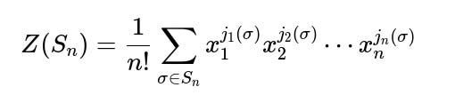
Yes. The cycle index polynomial for the symmetric group can be used to extract expected counts of cycles of various lengths:
The cycle index polynomial for the symmetric group Sₙ is

where j_k(σ) is the number of k-cycles in the cycle decomposition of σ.
We can find the expected value of jₖ(σ) by differentiating and setting x₁ = x₂ = … = 1. This approach yields that the expected number of k-cycles is 1/k.
The 2-cycle case is simply 1/2, matching our probability-based approach.
Pitfalls or deeper concerns:
The cycle index polynomial might be overkill for a simple question about 2-cycles, but in advanced combinatorics interviews, demonstrating awareness of it is beneficial.
One must ensure they handle the factor of 1/n! properly and the combinatorial expansions correctly. Mistakes in symbolic manipulation can lead to wrong results if done hastily.
If we interpret each “swap” as a random match in a bipartite graph, can we unify this with a graph-theoretic interpretation?
Sometimes permutations are represented by a perfect matching between two sets of n labeled vertices (positions on the left and values on the right). A 2-cycle i ↔ j is then a situation where left node i is matched to right node j, and left node j is matched to right node i:
This is basically a 2-cycle between i and j in the sense that edges (i, j) and (j, i) appear simultaneously.
Analyzing expected edges in random bipartite matchings can connect to known results in random graph theory. Specifically, a random matching that picks exactly one perfect matching out of all possible ones is just a random permutation. The probability that i and j form that 2-cycle remains 1/[n(n-1)].
The advantage of this viewpoint is that it might generalize to partial matchings or different constraints. But for the standard scenario, it’s effectively the same argument.
Edge cases:
If the bipartite graph is not a perfect matching but some other random structure (e.g., each node can connect to multiple nodes), we break the permutation property. Then the probability or even the definition of a “swap” might be altered or ill-defined.
In network scenarios, real edges might be weighted or some edges might be forbidden. That again modifies uniformity.
Could the random variable for the number of 2-cycles ever be negative or have any strange boundary conditions?
While this might sound trivial, interviewers sometimes ask tricky “sanity checks”:
The number of 2-cycles can’t be negative. It’s a count of events. The minimum is 0 (a permutation with no 2-cycles).
The maximum count is ⌊n/2⌋, for the reason discussed about disjoint cycles. Any scenario outside that range indicates a misunderstanding or a miscalculation.
If we do any advanced expansions, we must ensure we never allow counts outside these logical boundaries. A candidate might inadvertently produce a formula that yields an impossible range if they handle dependencies incorrectly.
Pitfall:
Overcounting in code. If someone checks pairs (i, j) in a loop and increments the count for both (i, j) and (j, i), they’d double the result. The correct approach typically keeps i < j or i > j exclusively, or divides the final count by 2.
Another potential confusion: if code uses 0-based indexing incorrectly, it might shift the logic for what is considered a “swap.” Ensuring correctness in implementation is essential.
If an interviewer asks you to detail an alternative derivation not using indicator variables, could you approach it via counting arguments alone?
Yes, though indicator variables are the cleanest method, a direct counting approach is also possible:
Let X be the number of 2-cycles in the permutation. Summation of X across all permutations is the total number of pairs (i, j) that form 2-cycles across all n! permutations.
Each pair (i, j) with i < j occurs as a 2-cycle in exactly (n-2)! permutations. So if we consider all possible pairs i < j, that’s n(n-1)/2 pairs, each appearing (n-2)! times across the entire space of n! permutations.
Hence, the total count of 2-cycles across all permutations is [n(n-1)/2] × (n-2)!. Dividing by n! yields the average across permutations:
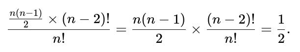
This method is effectively the same logic but framed as summing across permutations rather than using a probability argument for each pair individually.
Pitfall:
A candidate might forget to divide by n! or might incorrectly multiply the counts.
They might also forget the condition i < j, leading to a factor-of-two error if they double-count (i, j) and (j, i).
What if the interviewer wants an explanation of exactly why the probability for one pair (i, j) is 1/(n(n-1)), step by step?
Sometimes an interviewer will dig into the basics of uniform permutations:
Pick any permutation of n distinct elements uniformly from the n! possibilities.
To have i at position j and j at position i, we fix those two positions. That leaves (n-2)! ways to arrange the other (n-2) elements in the remaining (n-2) slots.
Hence there are (n-2)! permutations that yield i ↔ j.
Probability = (n-2)! / n!.
Simplify:

Pitfall:
Overlooking that we must choose distinct i and j. If i = j, the condition “i is in j-th position and j is in i-th position” collapses to a single position, not a 2-cycle. This is disallowed or is simply zero probability for a 2-cycle event since i must differ from j.
In code, mixing up position j (0-based) with index j (1-based) is a common error. The correct logic must align with a consistent indexing scheme.
Would the expected value be the same if we consider permutations of length n but only choose among permutations that have exactly one fixed point?
Yes, this is yet another conditional distribution problem. If we fix a scenario where exactly one element is in its correct position, then the rest is a distribution over permutations with that one fixed point. The presence of that single fixed point might slightly alter the probability of forming 2-cycles among the remaining n-1 elements. However:
We can define the restricted set of permutations: choose which element is in its correct position, and then the other n-1 elements permute among themselves in ways that might or might not form 2-cycles.
The detailed probability for i ↔ j might shift because i or j could be that fixed point, or neither, or some other scenario. Hence the total distribution is no longer uniform across all permutations. The resulting expected value can differ from 0.5.
Typically, as constraints accumulate (exactly one fixed point, or exactly two fixed points, etc.), the chance of 2-cycles can be re-derived using partial inclusion-exclusion or direct enumeration.
Edge case:
If the chosen fixed point is i, then i can’t participate in a 2-cycle i ↔ j. That reduces the possible 2-cycles for that i.
Over the entire distribution, we’d average out across which element is the fixed point. The final number might still be near 0.5 for large n, but it won’t be exactly 0.5.
How do we confirm quickly in an interview that no obvious mistakes were made in concluding the expected value is 0.5?
A quick sanity check:
For n = 2, the permutations are [1,2] and [2,1]. In the first, no 2-cycle because 1 is in position 1 and 2 is in position 2. In the second, 1 ↔ 2 is a 2-cycle. So the total number of 2-cycles across all permutations is 1, and there are 2 permutations, so the average is 1/2. That perfectly matches the formula.
For n = 3, we have 6 permutations. Only one of them is [2,3,1], which has no 2-cycle. Actually, we can systematically check each:
[1,2,3]: no 2-cycle.
[1,3,2]: only 2 ↔ 3? Actually, 2 is in position 3, but 3 is in position 2, so that’s a 2-cycle. So count = 1.
[2,1,3]: this has 1 ↔ 2 in positions, so count = 1.
[2,3,1]: check if 3 ↔ 2 or 1 ↔ something. Actually, 2 is in position 1, 3 is in position 2, 1 is in position 3, so we have no 2-cycle (2→1, but 1→3, 3→2 is a 3-cycle).
[3,1,2]: check 3 is in pos1, 1 in pos2, 2 in pos3. That’s no 2-cycle; it’s a 3-cycle again.
[3,2,1]: check 3 in pos1, 2 in pos2, 1 in pos3. That’s no 2-cycle (1→3, 3→1 is not correct because 3 is at index1 but index3 is 1, so actually that is a 2-cycle. Wait, carefully: index1 is 3, index3 is 1. In 1-based sense, position1 has 3, position3 has 1, so that’s 3↔1? But we also need that position1 has 1 if we want 1↔3, which is not the case. So no 2-cycle).
Counting carefully might lead to a total of 2 or 3 among the 6 permutations. Dividing by 6 should yield an average near 0.5. This small check is consistent with the theoretical expectation.
Pitfall:
Confusion from indexing or from incorrectly enumerating permutations. It’s easy to mislabel positions. The main point is that small cases indeed confirm the theoretical 0.5.
The interviewer might watch how systematically you check permutations. Rushing can lead to an incorrect conclusion, so it’s better to be systematic or rely on code or well-known results.

