
ML Interview Q Series: Expected Value & Std Dev for Finding All Aces: A Geometric Distribution Approach

Browse all the Probability Interview Questions here.
You have a thoroughly shuffled deck of 52 cards. Each time you pick one card from the deck, you replace it and reshuffle thoroughly. You repeat this process until you have seen all four different aces. What are the expected value and the standard deviation of the number of draws needed?
Short Compact solution
Consider the draws until the jth new ace has been observed as a geometric random variable X_j with success probability p_j = (4 - (j - 1)) / 52 for j = 1,2,3,4. The total number of draws is X_1 + X_2 + X_3 + X_4. From properties of geometric random variables:
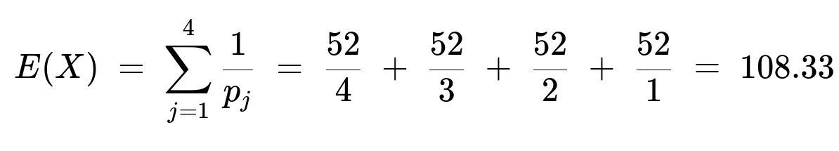
The expected value of each X_j is 1 / p_j.
The variance of each X_j is (1 - p_j) / p_j^2.
The random variables X_1, X_2, X_3, and X_4 are independent.
Hence, summing up:
E(X_1 + X_2 + X_3 + X_4) = 52/4 + 52/3 + 52/2 + 52/1 = 108.33
And
σ(X_1 + X_2 + X_3 + X_4) = 61.16
Comprehensive Explanation
Motivation and Setup
We are drawing cards from a deck of 52 cards with replacement. That means after each draw, the card is put back, and the deck is fully shuffled. We want to know how long it takes to observe all four distinct aces at least once.
The problem can be viewed as a form of the “coupon collector” scenario, but with only 4 distinct “coupons” (the four suits of aces) instead of 52. Each new ace we try to collect appears in the deck with a probability that depends on how many aces we still have not seen.
Decomposing the Time into Geometric Random Variables
Let X_j be the number of draws it takes from the time we have seen (j-1) distinct aces until we see the jth distinct ace. When we have already collected (j-1) distinct aces, there remain (4 - (j-1)) unseen aces in a deck of 52 cards. Therefore, on any single draw, the probability p_j of drawing one of the yet-unseen aces is (4 - (j - 1)) / 52.
Because each draw is independent (due to replacement and shuffling), X_j follows a geometric distribution with success probability p_j. A geometric random variable with success probability p has:
Expected value = 1/p
Variance = (1 - p)/p^2
Since the total time to see all four aces is X = X_1 + X_2 + X_3 + X_4, the expectation and variance of X are the sums of the individual expectations and variances (because X_1, X_2, X_3, and X_4 are independent).
Expected Value Calculation
The success probabilities for each stage j = 1,2,3,4 are p_1 = 4/52, p_2 = 3/52, p_3 = 2/52, p_4 = 1/52.
Hence, the expected number of draws to get the jth new ace is 1/p_j. Summing these:
where:
52/4 accounts for the time to get the first new ace (success probability 4/52),
52/3 accounts for the time to get the second new ace (success probability 3/52),
52/2 accounts for the time to get the third new ace (success probability 2/52),
52/1 accounts for the time to get the fourth new ace (success probability 1/52).
Variance and Standard Deviation
For each geometric random variable X_j:
Variance(X_j) = (1 - p_j) / p_j^2.
Therefore,
Var(X) = Var(X_1 + X_2 + X_3 + X_4) = ∑ Var(X_j) = ∑ (1 - p_j) / p_j^2.
We then take the square root of Var(X) to get the standard deviation σ(X). Numerically, this is computed to be approximately 61.16. In a more explicit form:

Practical Insight
On average, we need around 108 draws to see all four aces if each draw is from a thoroughly shuffled deck with replacement.
The high standard deviation of about 61 reflects that in some trials you may get the missing aces fairly quickly, while in other trials it can take substantially longer, especially for the last missing ace.
Simulation Example in Python
Below is a quick simulation using Python to verify these results empirically:
import random
import statistics

def simulate_draws(num_simulations=10_000_00):
    results = []
    for _ in range(num_simulations):
        seen_aces = set()
        count = 0
        while len(seen_aces) < 4:
            count += 1
            card = random.randint(1, 52)  # represent each card by an integer 1..52
            # Suppose aces are represented by 1, 2, 3, 4 for Ace of Clubs, Diamonds, Hearts, Spades
            if card in [1, 2, 3, 4]:
                seen_aces.add(card)
        results.append(count)
    return statistics.mean(results), statistics.pstdev(results)

avg_draws, std_dev = simulate_draws()
print("Simulation Mean:", avg_draws)
print("Simulation Std Dev:", std_dev)
This simulation draws a card uniformly at random, checks if it is one of the four distinct aces, and stops once all have been seen.
Over a large number of simulations, the empirical mean and standard deviation will converge to the theoretical values of approximately 108.33 and 61.16, respectively.
Possible Follow-up Questions
How do we generalize this result if we want to observe all k specific cards in a deck of size N?
To find the expected number of draws with replacement to see all k distinct cards, we note the success probability for collecting the jth new card is (k - (j - 1)) / N for j = 1,2,...,k. Summing the inverse of these probabilities gives:
E = N/k + N/(k - 1) + ... + N/1.
A similar approach applies for the variance, summing the individual variances of each geometric stage.
Does the result change if we do not replace the cards back into the deck?
Yes, that becomes the classical “no-replacement” coupon collector scenario, which has a different distribution. In that case, each draw changes the composition of the deck. The probabilities for each new draw are not independent in the same way, and you cannot model each stage as a geometric random variable with a fixed probability. The analysis becomes more complicated, often approached with hypergeometric distributions rather than geometric distributions.
Why is there such a large standard deviation?
When collecting rare items (especially when nearing the final “missing” item), the waiting time can be quite prolonged if you are unlucky. This skewed distribution of waiting times, common in coupon collector type problems, results in a relatively high variance (and hence high standard deviation).
If I wanted to reduce the variance in a real application, is there a strategy to do that?
In practical scenarios (though not typically with playing cards), if you can influence the sampling procedure to diversify your “draws” or try to avoid already-collected items, you might reduce the total time to collect all items and lower the variance. In classical deck-drawing with replacement, however, there is no straightforward way to reduce variance since the process is memoryless and each card is equally likely at each draw.
How does this relate to the classical Coupon Collector’s Problem for 52 distinct cards?
In the classical Coupon Collector’s Problem with 52 different cards, you would compute the expected time to collect all 52 distinct cards as 52(1/52 + 1/51 + ... + 1/1). That sums to approximately 236.0. The standard deviation can also be computed, but it’s significantly larger in that case. Here, we are only dealing with 4 of the 52 cards, which simplifies the math considerably.
In an interview, demonstrating your ability to generalize the reasoning, articulate edge cases (like replacement vs. no replacement), and connect to known distributions shows a strong understanding of probability, statistics, and random processes.
Below are additional follow-up questions
What if we only need to see some subset of aces (for instance, exactly two of the four aces) before stopping?
In some real-world scenarios, you might not need all four aces, but only a subset, such as the Ace of Spades and Ace of Hearts. This changes the success probability because you only care about 2 distinct targets rather than 4. In this subset case:
The probability of success on any given draw is (number_of_remaining_unseen_aces) / 52.
You would then define two geometric phases instead of four (one for the first unseen ace, and one for the second).
The expected number of draws becomes 52/2 + 52/1 if you only need 2 distinct aces.
A subtlety here is that once you have collected one of the aces, you no longer care about the other two. That can mean fewer overall draws, but it also might result in a situation where you keep drawing the same ace repeatedly before seeing the other one you actually need.
A potential pitfall arises if you are not fully certain which particular aces you are targeting. For instance, if you decide mid-way to change which subset of aces matters to you, you can no longer treat the geometric stages as purely independent or with a fixed probability. Always ensure the target set is fixed from the start to apply the standard geometric argument reliably.
What if each card draw is biased or not perfectly random?
In the classical math formulation, each card draw is assumed to be a uniform draw from the 52 cards. But in many real systems, “shuffling” might not be perfectly uniform. If certain cards are more likely to appear than others:
The probability of drawing an unseen ace changes in ways that are not captured by the simple fraction (4 - (j-1))/52.
You might systematically get certain aces more quickly and have longer waiting times for others.
The geometric distribution assumption breaks down because the success probability is no longer constant on each draw.
An edge case here is if the bias is unknown or if it changes over time (e.g., the shuffling mechanism gets better or worse). Then the distribution of the waiting time to see each new ace can be non-stationary. A robust approach might involve modeling the unknown probability with a Bayesian prior or performing repeated calibrations to estimate if some suits are overrepresented.
Could we use a stopping rule that is not just “wait until all four aces have been seen,” and how does that affect our analysis?
In some practical applications, you might use an alternative stopping rule—say, “stop after N draws regardless, but check how many distinct aces you have seen by that time.” This changes the nature of the problem:
Instead of focusing on the time to collect all 4 aces, you might be interested in the probability of having seen all 4 within N draws.
You can then evaluate the distribution P(X ≤ N) for X being the number of draws needed.
This probability can be derived from the negative binomial or geometric models, but the direct question of “expected time until the last ace” becomes a slightly different question of “distribution of how many distinct aces you have after N draws.”
A pitfall is that if you decide partway through to switch from the “all four aces” stopping rule to a fixed “N draws” stopping rule, your original geometric-based estimates of time and variance might not hold. You need a fresh calculation based on whichever stopping rule you finally adopt.
How would the Central Limit Theorem (CLT) apply if we repeat this experiment many times?
While each individual experiment (collecting all four aces) has a somewhat skewed distribution, if you repeat the experiment a large number of times and record the total draws X for each experiment:
By the CLT, the distribution of the sample mean of X’s over many repeats would approximate a normal distribution for sufficiently large sample sizes.
However, the distribution of X itself within a single experiment remains heavily skewed toward larger values because of the possibility of waiting a long time for the last ace.
A subtlety emerges if the number of repeated experiments is only moderate. The empirical distribution might still show heavy tail behavior and not look bell-shaped. Misinterpretation of partial data can lead to underestimating how often extremely large waiting times can occur.
What happens if we extend to multiple sets of aces—like trying to see all four aces twice each?
Sometimes, problems are extended to requiring multiple copies of each “coupon.” For instance, you might need to collect each of the four aces two times (with replacement in between). Now, you don’t only need to see each unique ace once; you must see them twice each:
The success criterion in each geometric phase is more complicated because, after the first time you see a particular ace, you still need to see that same ace once more.
You might treat each “slot” you need to fill as an item in a coupon collector puzzle. With 4 aces needed 2 times each, you effectively have 8 “slots.”
However, each draw still has probability 4/52 if you have 8 needed slots, then 3/52 if one slot is filled (but still 7 remain), etc. The order in which you fill the duplicates for each particular ace complicates the direct formula.
A pitfall is overapplying the simpler geometric approach to a scenario where you need duplicates. You might attempt to sum 1/p for each slot (which can still work in a modified form), but the state transitions can get tricky. A more rigorous approach involves enumerating states for how many times each ace has been collected.
How do we handle real scenarios where we might be looking for a more granular distribution rather than just mean and standard deviation?
In many data analytics or machine learning contexts, you might not only need E(X) (the expected time) and σ(X) (the standard deviation). You could need the entire distribution function for planning or risk assessment. For instance:
You might want to know the probability that X is less than some threshold T: P(X < T).
This can be important in planning scenarios, like how many draws you can afford in a time-constrained situation.
To find P(X < T), you need the cumulative distribution function (CDF) for X. For the sum of four independent geometric random variables, you can convolve their respective distributions, but that is more intricate than simply summing means and variances. A pitfall is incorrectly assuming that a normal approximation is accurate for small sample sizes. The distribution is discrete and skewed, so direct computations or approximations for the negative binomial form may be more accurate.
Do any real-world complexities (like partial memory or partial knowledge of the deck) invalidate the geometric assumption?
In practice, individuals might recall which card they drew last time, or the shuffle might not be thorough. That partial knowledge can produce correlations between draws:
If you know you drew an Ace of Spades on the previous draw, you might (incorrectly) suspect you’re less likely to get Ace of Spades the next time if you don’t trust the shuffle.
If the shuffle is genuinely perfect, then knowledge of the last draw does not help. But many real decks are not perfectly random after a single shuffle, so the geometric assumption of “constant probability of success each draw” might break.
A subtlety here is that even partial knowledge about the system can produce biases if the participants (or the algorithm) adapt their behavior. Ensuring true randomness is crucial for the geometric model to hold.
If we track not only whether we have seen an ace, but also how many times each specific ace has shown up, does that impact the number of draws needed to confirm we have four distinct aces?
If you meticulously track each ace, you might realize you have drawn Ace of Spades multiple times but are still missing Ace of Diamonds. This doesn’t directly change the expected number of draws to see all four, but it does inform you about which ace you are missing at any stage:
The knowledge of which particular ace is missing clarifies that the probability of success is 1/52 when you are down to just 1 unseen ace (the missing one).
In a scenario with less detailed tracking (maybe you only track “how many total aces have I seen so far?” but not which suits), you could become confused about whether you’ve actually seen the Ace of Diamonds or not.
A real-world pitfall is that partial data can lead you to overestimate or underestimate how many unique aces you have found so far. This confusion can cause you to stop drawing too early or keep drawing longer than necessary. In a purely mathematical setting with perfect memory, it doesn’t affect the distribution of X, but in an operational setting, it might cause errors in evaluating the true stopping time.