
ML Interview Q Series: Expected Value for All Die Faces: The Coupon Collector Problem Explained.

Browse all the Probability Interview Questions here.
How many throws of a fair six-sided die should you expect on average so that all six faces will have appeared at least once?
Short Compact solution
Let the current count of unique faces observed be denoted by k (ranging from 0 to 5). Whenever k distinct faces have already shown up, the probability of rolling a new face on the next throw is (6−k)/6. The expected number of additional throws needed to see the next new face follows a geometric distribution with success probability (6−k)/6. Hence, its mean waiting time is 6/(6−k). Summing these waiting times over k from 0 to 5:
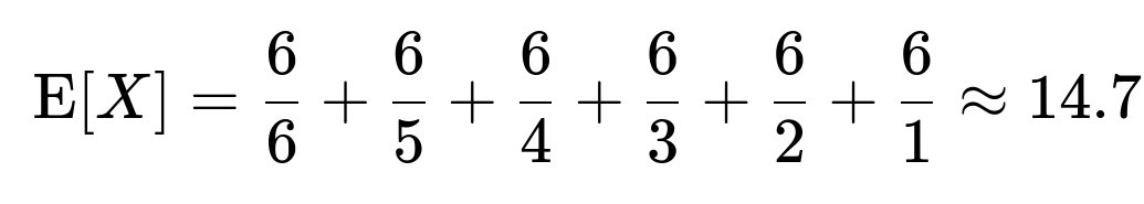
That total is approximately 14.7 throws.
Comprehensive Explanation
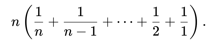
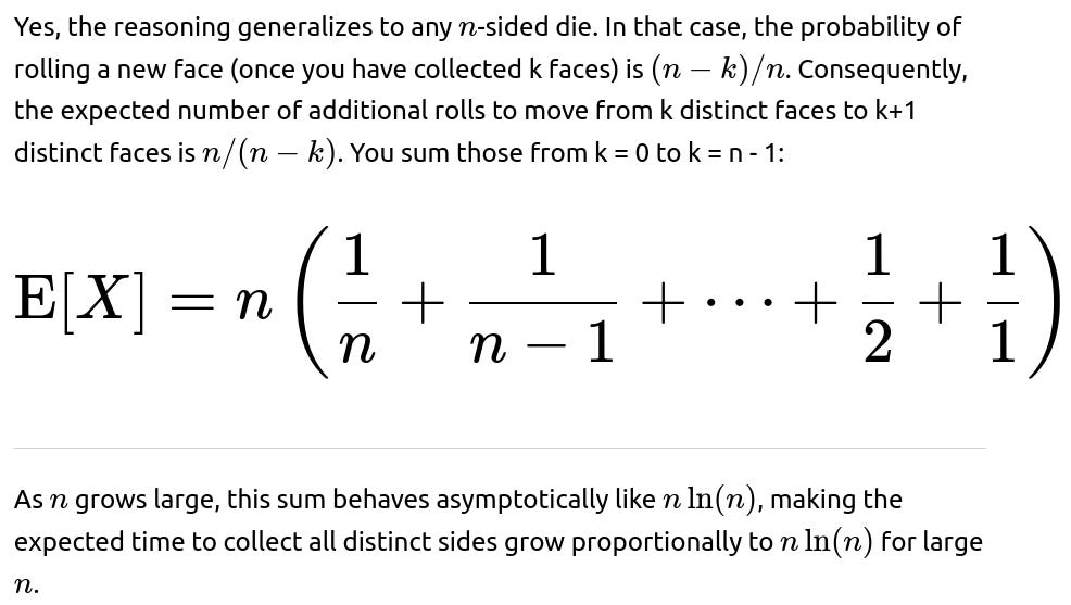
The problem of finding the expected number of rolls to see each face of a fair six-sided die at least once is a classic form of what is commonly called the Coupon Collector’s Problem. In general, if you have n distinct “items” (in this case n=6 sides of the die), the expected number of independent trials to collect all n items once is
For a six-sided die, we let n=6. The reasoning can be broken down into the stages of collecting new faces:
Initially, no faces are observed (k = 0). The first roll immediately shows a new face (k = 1). Once you have k distinct faces, the probability of seeing a new face on the next roll is (6−k)/6. Because each roll is independent, you can model the time to get from k distinct faces to k+1 distinct faces as a geometric random variable with parameter (6−k)/6. The mean of that geometric distribution is 6/(6−k). You then add these mean waiting times from k = 0 up to k = 5.
Concretely:
Going from 0 to 1 distinct face: you always succeed on the first roll, so the expected number of rolls is 6/6=1.
Going from 1 to 2 distinct faces: success probability is 5/6, so the expected waiting is 6/5.
Going from 2 to 3 distinct faces: success probability is 4/6, so the expected waiting is 6/4.
Going from 3 to 4 distinct faces: success probability is 3/6, so the expected waiting is 6/3.
Going from 4 to 5 distinct faces: success probability is 2/6, so the expected waiting is 6/2.
Going from 5 to 6 distinct faces: success probability is 1/6, so the expected waiting is 6/1.
Summing these gives a well-known harmonic structure:
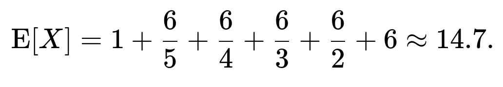
Hence, on average, it takes roughly 14.7 throws of a fair six-sided die to see all six faces at least once.
Follow-up question: Why is each stage modeled with a geometric distribution?
This arises from the memoryless property of independent die rolls. When you already have k distinct faces, the event of rolling a “new” face on the next roll has a fixed probability of (6−k)/6. Each roll is an independent trial with that fixed probability of “success” (i.e., seeing a new face). For a geometric distribution, the number of trials until the first success has an expected value of 1/p, where p is the success probability per trial. That is the key to each stage in the summation.
Follow-up question: What if the die is biased?
In the biased scenario, each face could have a different probability of appearing. Then the probability of seeing a new face at each stage is no longer simply (6−k)/6. Instead, you would need to account for whichever faces have not yet been observed and sum up their probabilities. The waiting time calculation becomes more involved, since the next “new” face might not arrive with a single uniform probability. In principle, you could still treat it as a “collect all distinct items” problem, but the expected time would require solving a more general form of the Coupon Collector’s Problem with non-uniform probabilities. One can use techniques like Markov chains to derive the expected time, but there is no simple closed-form expression analogous to the uniform case.
Follow-up question: What about the distribution of the number of rolls, not just the mean?
Although we commonly focus on the expected value, the full distribution is also of interest. For the uniform (fair) case, one can derive exact or approximate probabilities for the number of throws needed. This involves convolving the geometric distributions at each stage or can be analyzed via a Markov chain that tracks how many faces have been collected. It can be shown that, while the mean is about 14.7, there is a certain variance that allows for times both much shorter and much longer than that expected value. Often, people employ either direct enumeration methods or use a Markov chain approach to find the entire probability mass function.
Follow-up question: How can we verify these results empirically?
We can run a simulation in Python that repeatedly rolls a fair six-sided die until all faces have been seen, and then record how many rolls it took. Averaging over many trials gives a Monte Carlo approximation to the expected number of rolls. A simple code snippet might look like this:
import random

def simulate_dice_rolls(num_experiments=1_000_00):
    total_rolls = 0
    for _ in range(num_experiments):
        seen_faces = set()
        roll_count = 0
        while len(seen_faces) < 6:
            face = random.randint(1, 6)
            seen_faces.add(face)
            roll_count += 1
        total_rolls += roll_count
    return total_rolls / num_experiments

print(simulate_dice_rolls(1_000_00))
If you run this enough times (for example, one million experiments), you should see the average number of rolls converge to a value near 14.7.
Follow-up question: Does this approach generalize if we have more than six sides?
Below are additional follow-up questions
What if we are only interested in collecting a subset of the faces, not all six?
In some variations of this problem, one might only want to see three specific faces (e.g., faces 1, 3, and 5) rather than all six. This changes the success probability at each stage:
Only the faces in the desired subset are relevant.
Once you have k of the needed faces, there remain (subset_size - k) faces left to see.
The probability of rolling a new face from that subset depends on how many are still unseen among the subset, divided by 6.
Potential Pitfalls and Edge Cases:
Overcounting rolls: One might incorrectly assume the probability to see each new face remains constant, but it should be updated based on how many subset faces remain unseen.
Larger subsets versus smaller subsets: As the subset_size approaches 6, the problem converges to the standard coupon collector. For very small subsets, the expected time can be considerably shorter.
Real-world scenario: If someone is only looking for certain outcomes (like collecting only certain Pokemon cards out of a set), sometimes they overestimate how quickly they can achieve their smaller collection by using the logic for all items.
How does the presence of a stopping rule or budget constraint affect the expected time?
In practice, one might set a limit on the number of rolls (“we will only roll 15 times and then stop”). If we haven’t collected all sides by that time, we stop regardless. This introduces a censored or truncated scenario in which the random variable is effectively cut off at a certain threshold:
The expected time if we had infinite rolls is about 14.7. But if we have a stopping rule at, say, 10 rolls, the probability of having all faces by then is significantly less than 1.
The unconditional expectation might no longer apply because we don’t continue rolling if we reach the budget limit.
Potential Pitfalls and Edge Cases:
Misinterpreting the average: With a strict stopping rule, you can only say “the expected value if allowed to roll indefinitely is ~14.7.” Once you cap the roll count, you need to re-calculate the expected “observed count of distinct faces” by 10 rolls.
Unexpected real-world constraints: In manufacturing or testing contexts, sometimes there’s a limited number of trials before shutting down a line or moving on. Calculations must then incorporate that finite horizon.
Could we speed up the process by rolling multiple dice simultaneously?
An interesting extension is rolling multiple dice in parallel each time-step. Instead of a single independent trial, you might roll m dice per round:
The probability that a new face appears in a single round can be higher if you check all m dice for a previously unseen face.
Analyzing the expected time then involves considering the probability of obtaining at least one new face in each round, given that you have currently observed k faces.
Potential Pitfalls and Edge Cases:
Overlapping successes in the same round: If multiple new faces show up in the same roll, you might jump from k distinct faces to k+2 or more in a single round. Accounting for that can be more complicated than the single-die scenario.
Correlation in dice outcomes: Typically, if the dice are fair and rolled independently, each face is equally likely on each die. However, in some real-world situations, certain rolling methods might produce subtle correlations. That would further complicate the analysis.
Resource constraints: Rolling many dice in real life might be feasible, but in certain computational or experimental settings, “parallelization” might not truly reduce the wall-clock time or might have overhead.
How does the analysis change if each roll has some chance of being misread or lost?
In real experiments or data collection, you might occasionally fail to record the result of a roll. For instance, sensor glitches or human errors might cause you to miss the outcome of a roll:
If a result is missed entirely, it’s as though that trial never happened. You effectively don’t update which faces have been seen, so you remain at k distinct faces.
The probability of advancing from k to k+1 distinct faces changes, and the effective number of “usable” rolls is less than the total number of physical rolls.
Potential Pitfalls and Edge Cases:
Overlooking partial knowledge: Perhaps you see the outcome but can’t fully confirm the face. Some partial-credit approach might be needed if the face is recognized as “probably a 3 or a 4” but not certain.
Real-world reliability: In an industrial or sensor-based environment, the probability of missing a reading might not be negligible. Failing to incorporate this error can yield an underestimate of the real expected time.
Are there scenarios where the collecting process can regress?
In standard coupon collector problems, once you collect a new face, you never “lose” it. However, in certain dynamic or interactive processes, one could lose the “benefit” of having collected that face if conditions change or if the “collection” can expire. For instance, consider a scenario where each face is only “valid” for a limited time:
The concept of collecting all faces might be replaced by having all faces observed within a short rolling window.
This can introduce a Markov chain with states that fluctuate more than in the classic scenario, so the expected time to hold all six faces simultaneously changes drastically.
Potential Pitfalls and Edge Cases:
Overlooking the need to re-obtain a face that has “expired”: If each newly collected face has a timer, the problem can reset partially.
Misestimating probabilities if the “loss” mechanism is not clearly random: If the chance of losing a face depends on external factors, the entire process can deviate from the standard geometric assumptions.
How do we handle the situation where the die is replaced after each roll with a potentially different die?
Sometimes, rather than rolling one consistent fair die, you might have a bag of different dice, each with possibly distinct probability distributions (maybe each has a different weighting):
On each roll, you draw a random die from the bag, roll it, and see its outcome.
The probabilities of seeing a new face are no longer simply (6−k)/6. They depend on which die is drawn and how that particular die is weighted.
If the selection of the die is also random, you must average across the distribution of dice.
Potential Pitfalls and Edge Cases:
Inadvertent assumption of uniform distribution: If you assume each die in the bag is equally likely to be chosen, but in practice some dice might be chosen more often, this skews the distribution of observed faces.
Distinguishing which die produced which outcome: If you do not track which die was used for each roll, you might have less information about the underlying probabilities.
Could the order in which we see the faces matter?
If the requirement is not simply “see all faces at least once,” but rather “see all faces in a particular order,” then the expected time changes drastically:
For instance, if you need to see the face 1 first, then face 2, then face 3, and so on up to face 6 in that exact sequence, each success probability becomes more restrictive at each stage.
For face 1, any roll that does not show 1 is not progress, but seeing 2, 3, 4, 5, or 6 is effectively useless until you get 1.
Potential Pitfalls and Edge Cases:
Starting sequences: The probability of rolling your next required face is 1/6 if you haven’t seen that face yet. But partial sequences don’t help you unless they match the required order.
Repeats that are out of order: If you’re waiting for face 2 but keep rolling face 1, it doesn’t advance the sequence. Such scenarios can significantly increase the expected time compared to the standard coupon collector problem.
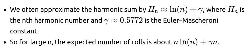
Are there extensions involving a large number of faces and approximations?
When the number of faces n is very large, exact summation of harmonic terms can be time-consuming or analytically unwieldy:
Potential Pitfalls and Edge Cases:
Heavy use of asymptotic approximations can hide constant factors that are still large enough to matter in real-world scenarios if n is big but not astronomically big.
If the distribution is not uniform, these approximations can be off by a large margin.
Could external feedback loops alter the probabilities after each roll?
Imagine a scenario where each time you roll a face you already have, you slightly adjust your rolling method, possibly biasing future rolls:
This breaks the assumption of independence across rolls because now the probability distribution for subsequent rolls depends on prior outcomes.
The standard coupon collector analysis does not hold, as the process is no longer memoryless in the standard sense.
Potential Pitfalls and Edge Cases:
Overcorrection: The feedback mechanism could become so strong that it overcompensates and makes seeing certain faces either too frequent or too rare.
Implementation details: In real dice rolling, subtle differences in how you throw the die can create small biases, though usually not large enough to systematically shift probabilities unless the dice or the environment is significantly altered.