
ML Interview Q Series: Expected Value Optimization for Risky Box Selection with All-or-Nothing Stakes.

Browse all the Probability Interview Questions here.
13E-7. Eleven closed boxes are put in random order in front of you. One of these boxes contains a devil’s penny and the other ten boxes contain given dollar amounts a_1,…,a_{10}. You may mark as many boxes as you wish. The marked boxes are opened. You win the money from these boxes if the box with the devil’s penny is not among the opened boxes; otherwise, you win nothing. How many boxes should you mark to maximize your expected return?
Short Compact solution
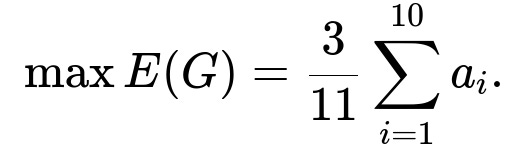
The expected value of your total gain E(G) can be written as:
where m is the number of boxes you choose to mark. Treating m as a continuous variable in [0, 11], the function m(1 - m/11) achieves its maximum at m = 5.5. Since m must be an integer, the optimal choices are m = 5 or m = 6. Substituting m = 5 or m = 6 into the expression for E(G) yields the same maximal expected gain, specifically:

Hence, marking either 5 or 6 boxes maximizes the expected return, with m = 6 being more “risky” in a probabilistic sense.
Comprehensive Explanation
Setting up the problem
We have 11 boxes total:
1 box contains a devil’s penny.
10 boxes contain dollar amounts a_1,…,a_{10}.
We do not know which box contains the devil’s penny. These boxes are placed in a random order in front of us, and we are allowed to pick (or “mark”) any number m of them to open.
If the devil’s penny is among the m chosen (opened) boxes, we win nothing.
If the devil’s penny is not among the chosen boxes, we receive the sum of the dollar amounts from those chosen boxes.
Defining the random variables
Let X_k be the random gain from the k-th chosen box (k = 1,…,m). Define G as the total gain:
G = X_1 + X_2 + … + X_m
Each X_k depends on whether the devil’s penny is in that box or not. Because exactly one box has the devil’s penny, there is an m/11 chance that the penny is among the m chosen boxes (since the devil’s penny is equally likely to be in any one of the 11 boxes).
Key probabilistic steps
Probability that the chosen boxes contain no devil’s penny This probability is 1 - m/11.
Gain from the chosen boxes If the devil’s penny is not among the chosen boxes (which occurs with probability 1 - m/11), then each chosen box is one of the 10 boxes containing amounts a_1,…,a_{10}. Because we do not know which dollar amounts specifically appear in the chosen boxes if the devil’s penny is excluded, the conditional distribution of each chosen box’s amount can be treated as a uniform choice over a_1,…,a_{10}, giving an average gain of (1/10) * (a_1 + a_2 + … + a_{10}) per box.
Expected gain per chosen box Condition on whether the devil’s penny is among the chosen boxes:
If the devil’s penny is there, the gain is 0 for that entire selection.
If the devil’s penny is not there, the expected gain for one chosen box is (1/10) * sum_{i=1..10} a_i.
Since the probability of not having the devil’s penny among the chosen boxes is 1 - m/11, the expected gain for one chosen box is:
E(X_k) = 0*(m/11) + (1/10)*sum_{i=1..10} a_i * (1 - m/11).
Therefore, E(X_k) = (1 - m/11)*(1/10)*sum_{i=1..10} a_i.
Total expected gain Because there are m chosen boxes, and each has the same expected value E(X_k), the total expected gain is:

Maximizing the expected gain
Let’s view the part m(1 - m/11) as f(m). Interpreting m as a continuous variable, we can set up:
f(m) = m(1 - m/11) = m - m^2/11.
Its derivative is:
df/dm = 1 - 2m/11,
and setting it to 0 leads to 1 - 2m/11 = 0, giving m = 5.5. Since m must be an integer between 0 and 11, we test integers around 5.5, namely 5 and 6. Both yield the same maximum value of the product m(1 - m/11).
Hence, the maximal expected return occurs at either m = 5 or m = 6. Substituting m = 5 or 6 into the expression above gives the same maximum:

Because marking 6 boxes implies a slightly higher probability of choosing the devil’s penny, it is described as “riskier,” but the expected gains (averaged over many trials) are the same for m = 5 or m = 6.

Potential Follow-up Question 1
What if the amounts a_i are all different or follow some non-uniform distribution?
Even if the amounts a_1,…,a_{10} are not identical or not uniformly distributed, as long as there is no information allowing us to preferentially select certain boxes over others (i.e., we still have no bias about which box might contain the devil’s penny or which might contain a particular a_i), the expected value calculation remains the same. Each of the 10 monetary boxes is equally likely to be in any of the unchosen positions once we exclude the devil’s penny. Thus the conditional distribution for the chosen boxes (given that the devil’s penny is not among them) is effectively a uniform choice among the 10 money boxes. Therefore, the same result for the optimal number of boxes m holds.
Potential Follow-up Question 2
Could any knowledge of the amounts (say some a_i are very large compared to others) change how we choose boxes?
If you have absolutely no hint about which box might contain which amount (apart from the single devil’s penny), there is still no advantage in specifically selecting or excluding certain boxes. Each of the 10 money boxes is equally likely to appear in any chosen set that doesn’t contain the devil’s penny. Consequently, the same expected-value approach applies, and the best strategy (m = 5 or m = 6) does not change. In a more general setting where you have partial information (e.g., you suspect higher amounts might appear in certain boxes), you would have to adjust your strategy accordingly. But in this classic puzzle statement, all boxes and the distribution of amounts are symmetric from your perspective.
Potential Follow-up Question 3
How would you compute the variance or standard deviation of the gain?
From the screenshot we see that a more detailed expression for E(G^2) (the second raw moment) is:
(1 - m/11)*[m/10 * sum_{k=1..10} a_k^2 + (m(m-1)/10×9) * sum_{k,l=1..10, k≠l} a_k a_l].
Then the variance Var(G) = E(G^2) - [E(G)]^2, and the standard deviation is the square root of that variance. While the question focuses on maximizing the expected value, the variance analysis sheds light on the “risk” involved if you pick more boxes (i.e., the chance of ending up with zero goes up because the devil’s penny might be in one of your chosen boxes).
Potential Follow-up Question 4
How can we simulate this in Python to verify the theoretical expectation?
Below is a rough Python outline for a Monte Carlo simulation:
import random
import statistics

def simulate_gain(num_boxes_to_mark, a_values, trials=10_000_00):
    # a_values: list of length 10 containing a_1,...,a_{10}
    # One box out of 11 is the devil’s penny
    # The remaining 10 contain the amounts a_values
    # We run multiple trials and compute average (empirical) gain.

    gains = []
    for _ in range(trials):
        # Randomly shuffle the 'devil' + a_values
        # We'll represent them as a list: [None for devil's penny] + a_values
        items = [None] + a_values[:]  # One None for the devil's penny
        random.shuffle(items)

        # Mark num_boxes_to_mark of them randomly (by indices)
        indices_chosen = random.sample(range(11), num_boxes_to_mark)

        # Check if devil’s penny is among chosen
        if any(items[i] is None for i in indices_chosen):
            gains.append(0)
        else:
            # Sum the amounts of the chosen boxes
            gain_sum = sum(items[i] for i in indices_chosen)
            gains.append(gain_sum)

    return statistics.mean(gains)

if __name__ == "__main__":
    a_values = [10, 20, 30, 40, 50, 60, 70, 80, 90, 100]  # example amounts
    for m in range(1, 12):
        avg_gain = simulate_gain(m, a_values, 100000)
        print(f"m = {m}, Empirical Average Gain = {avg_gain}")
Running this simulation for various choices of m, you would see (after many trials) that marking 5 or 6 boxes gives the highest average return, matching the theoretical analysis.
Potential Follow-up Question 5
What if the devil’s penny could be placed with higher probability in certain boxes (not uniformly random)?
In that case, the underlying assumption of a uniform 1/11 chance is violated. You would then need to account for the prior probability that each box might contain the devil’s penny. The formula for expected gain would be altered to incorporate these different probabilities. Moreover, you might choose fewer or more boxes depending on how likely you think each box is to contain the penny compared to the potential gain in that box. This becomes a Bayesian optimization problem, rather than a straightforward uniform-probability puzzle.
All these extensions highlight the importance of carefully modeling assumptions about probabilities and distributions of monetary values. However, under the original puzzle conditions of uniform randomness, the simple derivation stands, and the optimal strategy is to mark 5 or 6 boxes.
Below are additional follow-up questions
What if there is a cost for marking each box? How does that affect the strategy?
If each box you choose to open comes with a cost (for instance, you must pay c dollars per box you mark), then the expected gain formula changes. Originally, if you mark m boxes, your expected return is E(G) = m(1 - m/11)(1/10)(sum of a_i). Now you would have to incorporate the total cost of marking those m boxes, which is m*c. That transforms your expected profit to:
Profit = E(G) - cost = m(1 - m/11)(1/10)(sum of a_i) - m*c.
From a mathematical standpoint, you would then maximize that new function of m. The cost term penalizes choosing a larger m, so you expect the optimal m to shift downward relative to the no-cost scenario. Precisely where it lands depends on the relative magnitudes of c and sum of a_i. You would do a derivative-based maximization, or simply evaluate for each integer m from 0 to 11 and pick the one that yields the highest net profit.
A subtle pitfall could be if c is so large that the optimal m might be zero, meaning you decide to mark no boxes at all, resulting in a guaranteed zero gain but no cost. Another pitfall is if c is small enough that it does not strongly deter you from picking more boxes, in which case you might still settle around m = 5 or m = 6.
What if the dollar amounts a_1,…,a_{10} are themselves random variables?
Suppose each box that does not have the devil’s penny contains a random payout A_i, drawn from some distribution (potentially different for each i, or even correlated). From a theoretical standpoint, you can still compute your expected gain, but it becomes:
E(G) = m * (1 - m/11) * E(A),
where E(A) is the expected payout of a single money box. If the A_i have different distributions, you might use the average expectation across those distributions, denoted by E(A). Provided you have no information about which random distribution is assigned to which box, the same combinatorial argument remains: you have a 1 - m/11 chance that you avoid the devil’s penny and then, on average, each box yields E(A). Hence the formula for E(G) is effectively the same in structure, except that now sum_{i=1..10} a_i is replaced by 10 * E(A). You still find m = 5 or m = 6 maximizes m(1 - m/11).
A subtlety arises when the distributions are not identical. If you knew which boxes have higher or lower expected payouts, you would target the higher ones preferentially. However, if you truly have no knowledge about which box is assigned which distribution, the symmetry argument holds and the same pick-5-or-6 rule applies in expectation.
What if you receive partial hints about which box might contain the devil’s penny before finalizing your choice?
A scenario might arise where you gain partial information or “hints” as the boxes are revealed or from an external clue (like, “the devil’s penny is more likely in the left half”). Once you have such information, the probability is no longer 1/11 for each box being the devil’s penny. You can then update your belief for each box. For instance, if you know that with high probability p a certain subset of boxes does not contain the penny, you can weight your choices accordingly.
A subtle pitfall is ensuring your Bayesian updates are correct: incomplete or incorrect use of the hint might lead to a suboptimal marking strategy. Another pitfall is overconfidence in the hint. If the hint is noisy, you need to reflect that uncertainty in your updated probability distribution.
How do we incorporate risk aversion instead of simply maximizing expected value?
In some real-world settings, you might care not just about the average return but also about the variability or the probability of receiving zero. If you are highly risk-averse, you might prefer to pick fewer boxes because that lowers the chance of selecting the devil’s penny (which yields a total loss). Conversely, a risk-neutral or risk-taking individual might still follow the m = 5 or m = 6 strategy to maximize expected value.
A common way to incorporate risk aversion is to adopt a utility function that penalizes big losses. For instance, if U(x) = ln(1 + x) or some concave function, you would maximize the expected utility rather than expected monetary gain. This might give a different optimal m. A subtlety: the more concave the utility function, the stronger the incentive to avoid the scenario where you get zero. As a result, the “best” m might shift to a value smaller than 5.
What if there are multiple devil’s pennies and multiple sets of money amounts?
Imagine an extension where there are d devil’s pennies among the 11 boxes. If you open any box containing a devil’s penny, you still lose everything. But now there might be 10-d boxes containing some money. That changes the probability that you are safe from devils, since the chance of picking at least one devil’s penny grows with both m and d. You would need to calculate:
P(“no devils picked”) = (11 - m choose d) / (11 choose d),
assuming all subsets of size d for the devil’s pennies are equally likely.
The expected gain for each box chosen (conditional on no devil’s penny chosen) becomes an average over the money boxes, which might total 10-d or still 10 depending on how the puzzle is phrased. A subtle pitfall is ensuring you correctly handle the combinatorial count for multiple devils. Another subtlety is how the money is arranged among the boxes if the total number of money boxes is now less than 10.
What if you can revise your choice in multiple stages?
In some games, you might open a subset of boxes first, see partial outcomes, then decide whether to open additional boxes. This scenario requires a dynamic approach where you update your probability estimates after observing partial information (like “we didn’t find the devil’s penny in these initial boxes, so it must be in the remaining ones with certain revised probabilities”).
The pitfall here is that the simple single-shot analysis of picking 5 or 6 boxes simultaneously does not necessarily apply. A multi-stage approach could yield a different optimal strategy because you can glean information as you go. For instance, if you open one box at a time, you could stop immediately if the returns so far are decent and the risk of hitting the devil’s penny is getting too high.
Could the identity or correlation between the boxes matter?
If for some external reason the boxes are not independent (e.g., certain boxes are known or suspected to hold higher amounts and also possibly more likely to hold the devil’s penny), then the assumption of uniform probability distribution no longer holds. You would need a joint probability model for (devil’s penny location, money distribution). If the amounts in certain boxes are correlated or the devil’s penny is correlated with certain box features, the strategy might require picking fewer boxes that have a high expected payoff or carefully balancing the chance of encountering the penny.
A subtlety is ensuring that correlation is properly accounted for. For instance, if the devil’s penny is more likely to appear in a box that might contain the largest money amount, you have to weigh the large reward against the higher chance of a total loss.
What if the game is repeated many times and you can track outcomes?
When repeated over multiple rounds, you might try to exploit patterns in how the devil’s penny is placed or in how the boxes are shuffled. If it truly is random and memoryless each time, your best single-round strategy is still the best multi-round strategy. However, if you suspect the house or the game host is placing the devil’s penny with some partial pattern, you might detect and exploit it.
A subtle pitfall is overfitting: you might see patterns in random data that don’t actually exist. Another pitfall is that even if there is a slight pattern, it could require many rounds to detect it reliably, and your net profit while searching for that pattern might not outpace the simpler single-round expected-value strategy.
What if you can physically inspect or “weigh” the boxes to deduce partial information?
Sometimes real-world games allow players to pick up or weigh boxes, claiming that the devil’s penny might be lighter or heavier than the money. That knowledge effectively breaks the uniform-likelihood assumption. You then have a new conditional probability model: if you can weigh each box, you might find strong evidence about which box contains the penny. If you can do so reliably, you might be able to mark all the money boxes while excluding the devil’s penny.
A subtlety is measurement noise: if the penny is only slightly lighter or heavier than certain money amounts, you cannot be completely certain. Another subtlety is if you are only allowed to weigh a subset of the boxes or weigh them in an aggregated manner. Each of these constraints changes how you calculate your updated probabilities and thus changes your marking strategy.
What if you value partial outcomes differently (e.g., a single high-valued box is worth more than several lower-valued boxes)?
If your payoff is not simply the sum of the amounts from the marked boxes—for example, maybe you only get the largest single box’s value among your picks or some special function of the marked boxes—then the original summation approach no longer holds. You must define a new “gain function” that captures how the values of chosen boxes translate into final payoff.
A subtlety is that picking more boxes might not linearly add up your gain if only the largest single box among your chosen ones matters. In such a scenario, you might place more emphasis on picking the box that potentially contains the highest single a_i, but weigh that against the risk of picking the devil’s penny. Another subtlety is dealing with ties or synergy among multiple boxes (e.g., you only gain the difference between the largest and second largest box). Each alternative payoff structure calls for a reevaluation of the probability-based cost-benefit analysis.
What if the payoff is multiplied by a factor if you avoid the devil’s penny?
Imagine a twist: if you avoid the devil’s penny among your m boxes, your final payoff is multiplied by some bonus factor b > 1. Then your expected gain becomes:
m(1 - m/11)(1/10)(sum of a_i)*b.
This simply scales the same function by b and does not shift the location of the maximum, meaning your optimal m still remains 5 or 6. A subtle point is that if b is extremely large, you might be more tolerant of the bigger risk associated with picking more boxes, yet the fundamental shape of the function m(1 - m/11) still peaks at 5.5, so the integer optimum remains unaffected by a constant multiplier.
A more nuanced twist might be that the factor b itself depends on how many boxes you pick or on which amounts they contain, which would complicate the standard formula and could shift the optimal m.