
ML Interview Q Series: Expected Value for Consecutive Wins in 1/k Probability Games using Linearity of Expectation.
Browse all the Probability Interview Questions here.
You play a sequence of s games, where s ≥ 2 is fixed. The outcomes of the various games are independent of each other. The probability that you will win the k-th game is 1/k for k = 1, 2, …, s. You get one dollar each time you win two games in a row. What is the expected value of the total amount you will get?
Short Compact solution
Define X_k as the amount you earn at the k-th game if it and the (k−1)-th game are both won, and 0 otherwise (for k = 2, …, s). Then the total amount you earn is the sum of X_k from k = 2 to s. By linearity of expectation, the expected total is the sum of E[X_k] over k = 2 to s. Since P(X_k = 1) = 1/[k(k−1)], it follows that E[X_k] = 1/[k(k−1)]. Hence,

Therefore, the expected amount you get is (s−1)/s.
Comprehensive Explanation
Defining the Random Variables
Let us denote by X_k the random variable that equals 1 if you win two consecutive games on the (k−1)-th and k-th trials, and 0 otherwise. We only define X_k for k = 2, 3, …, s, because you need at least two games to determine a pair of consecutive wins.
Linearity of Expectation
The total amount you earn from the s games is the sum of X_k for k = 2 to s. We denote this by T = X_2 + X_3 + … + X_s. The expected value of T can be written (by the linearity of expectation) as:

Computing E[X_k]
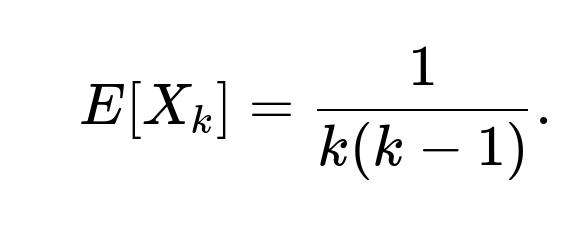
Because each game’s outcome is independent from the others, the probability of winning two consecutive games, i.e. P(X_k = 1), is the product of the probability of winning the (k−1)-th game and the probability of winning the k-th game. The (k−1)-th game is won with probability 1/(k−1) and the k-th game is won with probability 1/k. Therefore,
P(X_k = 1) = (1/(k−1)) * (1/k) = 1/[k(k−1)],
and so
Summing Up the Expectations
To find E[T], we sum E[X_k] from k = 2 to s:

This sum is well-known to telescope. Observe that:
1/[k(k−1)] can be rewritten as (1/(k−1)) − (1/k).
Hence, when we expand the series for k = 2, 3, …, s, most intermediate terms cancel out:
(1/1 − 1/2) + (1/2 − 1/3) + (1/3 − 1/4) + … + (1/(s−1) − 1/s).
All the interior terms cancel, leaving:
1 − 1/s = (s−1)/s.
Thus:

This completes the derivation that the expected total amount you earn is (s−1)/s.
Potential Follow-Up Questions
How does linearity of expectation apply when X_k variables are not mutually independent?
Even though the indicator variables X_k can be correlated (because winning the k-th game also affects X_{k+1}, and so on), the linearity of expectation does not require independence. Linearity of expectation holds for any set of random variables, regardless of whether they are independent or not. Specifically,
E(X_2 + X_3 + … + X_s) = E(X_2) + E(X_3) + … + E(X_s)
always remains true.
Could we have approached this problem with a different method, such as direct enumeration or Markov chains?
Yes. One might set up a small Markov chain with states that describe whether the last game was won or not, then track the expected number of transitions into the "two consecutive wins" state. However, such an approach requires more steps, whereas using indicator variables and linearity of expectation is more straightforward.
What happens in the edge case s = 2?
When s = 2, we have only two games:
Probability of winning game 1 is 1/1 = 1.
Probability of winning game 2 is 1/2.
X_2 = 1 if we win both games 1 and 2, which happens with probability 1 * 1/2 = 1/2. Hence the expected amount is 1/2. Our formula (s−1)/s gives (2−1)/2 = 1/2, which matches perfectly.
Could this logic be extended if the probability of winning each game was not 1/k?
Yes. If the probability of winning the k-th game is p_k (some general value), then P(X_k = 1) = p_{k−1} * p_k. Consequently, E[X_k] = p_{k−1} * p_k, and you would sum these values from k = 2 to s. You would not get a neat telescoping sum in general, but you would still use the same linearity-of-expectation principle:
E(T) = p_1 p_2 + p_2 p_3 + … + p_{s−1} p_s.
Practical Implementation: Simulation Example in Python
Below is an illustrative code snippet to simulate the scenario and empirically approximate the expected winnings. As s grows, the empirical average should approach (s−1)/s.
import random
import statistics

def simulate_earnings(s, num_simulations=10_000_00):
    results = []
    for _ in range(num_simulations):
        # Play s games
        wins = [(random.random() < 1/k) for k in range(1, s+1)]
        # Calculate total for consecutive wins
        total = 0
        for k in range(1, s):  # k is index 1-based
            if wins[k-1] and wins[k]:
                total += 1
        results.append(total)
    return statistics.mean(results)

s_value = 5
approx_expected = simulate_earnings(s_value)
theoretical = (s_value - 1) / s_value
print("Simulated expected:", approx_expected)
print("Theoretical expected:", theoretical)
In this code:
We generate s outcomes, each with its respective probability of winning.
We check consecutive outcomes for wins.
We repeat this experiment many times and average out the total earnings.
The variable
theoreticalcalculates the closed-form expression (s−1)/s.
Thus, both theory and simulation confirm that the expected value is (s−1)/s.
Below are additional follow-up questions
What if we want not only the expectation but the entire distribution of the total number of dollars won?
One might wonder how likely it is to earn exactly 0 dollars, exactly 1 dollar, exactly 2 dollars, and so on, across the s games. Although the expectation can be computed neatly using linearity of expectation, deriving the full probability distribution often requires accounting for all combinations of wins and losses.
Approach: We could model the process as a Markov chain with states indicating "did not win the previous game" or "won the previous game," together with a running count of how many times two consecutive wins have occurred. As s grows larger, the complexity grows, so the direct combinatorial approach would be quite involved.
Pitfall: When computing exact distributions, it is easy to overlook overlapping events, such as winning consecutive pairs (game 2, game 3) and (game 3, game 4). A naive enumeration might double-count certain scenarios or miss others.
Practicality: For moderate s, a dynamic programming approach can systematically track probabilities of reaching a certain count of consecutive-win occurrences by each game step. For large s, a simulation-based approach is often more practical if all we need is an approximation of the distribution.
How do we handle cases where s is very large, potentially approaching infinity?
In real-life applications, one might consider a long sequence of games. A natural question is how the result scales as s → ∞.
Behavior as s → ∞: The expected value (s−1)/s approaches 1 as s becomes large. Intuitively, when you play many games, on average you are likely to pick up close to 1 dollar per sequence because eventually the pairwise consecutive wins occur enough times relative to the number of games.
Deeper consideration: If s is extremely large, we might want to look at the law of large numbers or a limiting distribution. However, in this particular case, you only earn a 0/1 increment for each pair of consecutive wins, and each pair depends on specific probabilities. As s grows, the fraction of times you get consecutive wins might converge to some limit. The exact fraction is not the same as the total expected earnings divided by s (which would be ((s−1)/s)/s = (s−1)/(s^2)), but one might look at average earnings per game or per pair of games.
Pitfall: Over a very large number of games, small differences in probabilities can accumulate. If the probability of winning the k-th game was slightly misestimated or subject to some error, the overall expected payout could deviate more significantly than one might anticipate for small s.
What if the payoff changes after each pair of consecutive wins?
Sometimes, a follow-up scenario might involve a changing reward structure. For example, the first time you get two consecutive wins, you receive 1 dollar, but the second time, you receive 2 dollars, and so on.
Effect on the approach: The key difference here is that X_k can no longer be a simple Bernoulli random variable with a fixed payoff. Instead, the reward for the event "consecutive wins at times k−1 and k" could change over time.
Computation: We can still define indicator variables for consecutive wins but multiply those indicators by the appropriate payoff. For instance, let Y_k be the reward you get from your k-th consecutive win occurrence. The expectation is still the sum of E[Y_k] over k, but identifying the exact index k of consecutive-win occurrences (as opposed to the time index for the game) can be more involved.
Pitfall: Overlapping events and the order in which consecutive wins occur matter a great deal. This can no longer be handled by simply summing up probabilities for each pair, so a more sophisticated state-based or enumerative approach is required.
What if each win has an associated cost, and we want net expected value?
In a practical betting scenario, you might pay a certain fee or wager to play each game, so you want the expected profit rather than just the raw expected winnings.
Adjusting the result: Let c be the cost to play each game. Then you pay a total of s·c over the entire sequence. Your total winnings from consecutive wins are still random with expectation (s−1)/s. Hence, the expected net outcome would be (s−1)/s − s·c.
Pitfall: If c is large enough, it might overshadow the expected gains even though you have a decent chance of getting several pairs of consecutive wins. This can turn the game into a negative-expectation scenario.
Edge Cases: If c is dependent on k (for instance, a cost that changes each time you play), you would need to sum up all those costs and then subtract from your expected winnings.
Are there scenarios where the independence assumption might fail, and how would that change the analysis?
In real-life or certain game structures, the probability of winning the k-th game might depend on the outcomes of previous games (beyond just the probability of 1/k). For example, winning streaks might improve or worsen future winning chances.
Violation of independence: If the probability of winning a game changes based on past outcomes, you cannot simply multiply probabilities or treat them separately. A more complex model is required, potentially a Markov process or a more general dependence structure.
Impact on expected value: Linearity of expectation still applies, but P(X_k = 1) is no longer just 1/(k(k−1)). You must compute the correct probability of consecutive wins by carefully tracking the evolving probability of each outcome.
Pitfall: A naive approach might incorrectly continue to use 1/k as the probability of winning game k, ignoring the effect of past outcomes. This can lead to incorrect conclusions about expected values and distribution.
Could there be any numerical or simulation-based stability issues for large s in code implementations?
When we simulate or perform computations for large s, certain numerical issues might arise:
Floating-point errors: Probabilities like 1/k might become very small for large k, and summing a large number of tiny probabilities can introduce floating-point inaccuracies. Although 1/k by itself is not extremely small, in certain extended or more elaborate models, one might deal with tiny probabilities that cause precision issues.
Simulation horizon: If we simulate up to s = 10^6 or more, it might be computationally expensive and could lead to performance bottlenecks. Therefore, one must ensure the code is optimized, possibly vectorizing operations or relying on more advanced sampling techniques.
Pitfall: Rounding issues can accumulate if we keep incrementing floating-point counters in a loop for very large s. The final result might deviate from the theoretical value if the accumulation of floating-point error is not handled properly (though Python’s double precision typically handles sums of this scale relatively well in practice).
What if we require winning three games in a row, or a longer streak, to earn money?
A natural extension is to say: you only earn a dollar if you win k consecutive games. For our original problem, k = 2. But what if k = 3, 4, and so forth?
Generalizing: To earn 1 dollar for winning k consecutive games, define an indicator variable that checks the last k games. For instance, if you want 3 consecutive wins, you look at game indices i−2, i−1, and i, and check if each was a win.
Expected value: You can still use linearity of expectation, but each indicator variable now has probability (1/i) * (1/(i−1)) * (1/(i−2)) ... up to k factors. This is 1 / [i(i−1)(i−2) ... (i−(k−1))]. The summation becomes more complex, but can sometimes telescope for simpler forms like 1/k, 1/k−1, etc.
Pitfall: As k grows, the sum may not have a simple closed-form expression. Handling the edge indices (e.g., you cannot have 3 consecutive wins for i < 3) also needs care. The pattern of cancellation in the partial fraction decomposition might not be as straightforward.
Implementation detail: For k = 3, we would define something like X_i = 1 if the (i−2), (i−1), and i-th games are won, and 0 otherwise, for i ranging from 3 to s. The probability is 1 / [i(i−1)(i−2)], and the sum might or might not telescope cleanly, depending on the form of partial fractions.