ML Interview Q Series: Explain how gradient descent works and discuss why stochastic gradient descent is often preferred

📚 Browse the full ML Interview series here.
Short Compact solution
Gradient descent moves in small increments along the steepest descent direction to optimize a chosen objective function. Each move, known as a “step,” is scaled by the negative gradient of the function at the current parameter values. The stochastic form, commonly called stochastic gradient descent (SGD), replaces the exact gradient with an approximation obtained by randomly sampling a single data point (or a small subset) at every iteration. This reduces computational overhead for large datasets and is especially beneficial when data points are redundant or share similarities.
When using gradient descent, parameters are updated iteratively:
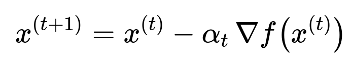
At each update, the negative gradient of the objective function is computed, scaled by a learning rate, and subtracted from the current parameter vector. Many common loss functions can be decomposed into sums over individual samples, but computing a full gradient every time can be expensive for huge datasets and can make the algorithm more prone to getting stuck in local minima or saddle points. By randomly picking a single example (or a small batch) to approximate the gradient, SGD delivers an unbiased estimate of the true gradient. Formally, if data points are assumed to be independently and identically distributed, the expected value of the stochastic gradient equals the actual full gradient.
Comprehensive Explanation
Gradient descent and stochastic gradient descent form the backbone of many machine learning and deep learning optimization routines. They are used to minimize an objective or loss function by iteratively refining a model’s parameters in the direction that most steeply reduces the loss.
Core idea of Gradient Descent
Gradient descent relies on the observation that the gradient of a function points in the direction of steepest increase. By stepping in the opposite direction of the gradient (that is, subtracting a gradient-related term), we gradually move parameters toward a local or global minimum of the objective function. Key considerations include:
Learning Rate (Step Size) This factor determines the magnitude of each update. If it is too large, the algorithm may overshoot the minimum and diverge. If it is too small, convergence can become slow or the algorithm can get stuck in suboptimal areas.
Loss Function Decomposition Many loss functions in machine learning are expressed as sums or averages of per-sample losses. For instance, when training a neural network on n samples, the overall loss might be:

In batch gradient descent, we compute the gradient of this entire sum (or average) at each iteration.
Convergence Criteria Common stopping criteria involve setting a maximum number of iterations, or stopping when changes to the loss or parameter updates become very small. Practical implementations also monitor validation metrics to avoid overfitting.
Rationale Behind Stochastic Gradient Descent
While gradient descent calculates the exact gradient based on all samples, stochastic gradient descent approximates the gradient using only one (or a small subset of) training sample(s) per update. This has several practical advantages:
Computational Efficiency Computing the gradient on a single sample or a small batch is significantly faster than summing over the entire training dataset. This makes SGD particularly useful when data is large enough to make complete passes prohibitively time-consuming.
Noise and Escaping Saddle Points Using only a random subset of data per update introduces noise into the parameter updates. Paradoxically, this noise can be advantageous, as it sometimes helps the model escape shallow local minima or saddle points and explore the parameter space more effectively.
Online Learning and Streaming Data In cases where data arrives in streams or in real time, stochastic updates allow the model to incorporate each new data point without waiting for the entire dataset to be processed.
Variants and Practical Concerns
Mini-Batch Gradient Descent Instead of using just one sample (pure stochastic) or using the entire dataset (batch), many practitioners choose a small batch size (like 32, 64, 128). This balances the noise from a single sample against the computational cost of a full batch, often yielding more stable updates while retaining the speed benefits of stochastic methods.
Adaptive Optimizers Optimizers like Adam, RMSProp, and Adagrad build on top of stochastic gradient descent by adapting the learning rate for each parameter during training. This can lead to faster convergence and more robust behavior in the presence of sparse data or large parameter spaces.
Learning Rate Scheduling The learning rate can be reduced over time according to a schedule (e.g., step decay, exponential decay) to help the model settle into local minima more gently after initially making large updates.
Initialization and Other Pitfalls Gradient-based methods are sensitive to initialization. A poor choice of initial parameters can make convergence slower or lead the algorithm to a suboptimal local minimum. Proper initialization strategies and normalization techniques (like batch normalization in neural networks) often improve gradient-based optimization performance.
Practical Example in Python
import numpy as np

# A simple function to represent the loss (e.g., f(x) = (x - 3)^2 ).
def loss(x):
    return (x - 3)**2

# Gradient of the loss
def grad_loss(x):
    return 2*(x - 3)

# Learning rate
alpha = 0.1
# Initial guess
x = 10.0

for i in range(100):
    # Compute gradient
    grad_val = grad_loss(x)
    # Update rule
    x = x - alpha * grad_val

print("Estimated solution:", x)
In a setting where each step stochastically selects data points from a large dataset, the line grad_val = grad_loss(x) would be replaced by an approximation of the gradient based on a random sample or mini-batch. In large-scale machine learning, the parameters x would be vectors or matrices instead of a single scalar.
Potential Follow-up Question: How do we choose a proper learning rate in practice?
A good learning rate is problem-dependent. Typical strategies include:
Using a fixed, small learning rate if the dataset and model are not too large, ensuring stable convergence. Employing a decaying learning rate schedule that starts bigger to make quick initial progress but decreases over time to refine the solution more gently. Using adaptive methods like Adam or RMSProp, which internally adjust the step sizes for different parameters.
Choosing too large a learning rate can cause the loss to diverge, while picking it too small can lead to very slow convergence. Practitioners often run multiple experiments with different values to find an optimal range, or use heuristics such as learning rate warm-up or scheduling algorithms that reduce the learning rate when validation performance plateaus.
Potential Follow-up Question: In what scenarios might stochastic gradient descent fail to converge?
Stochastic gradient descent can fail to converge or get stuck if:
The learning rate is too large and the parameter updates keep overshooting the optima. The model or loss function has very pathological curvature or complex non-convex regions filled with saddle points, making it tricky to settle into a good solution. The dataset is noisy or not truly i.i.d., causing misleading gradient estimates. Data preprocessing or feature scaling is not performed, leading to significantly unbalanced gradient updates across different dimensions.
In practice, techniques like momentum, adaptive learning rates, or careful data normalization can mitigate these challenges.
Potential Follow-up Question: Why is mini-batch gradient descent often considered a good middle ground?
Pure stochastic gradient descent updates parameters from a single data point at a time, which can cause unstable convergence if the dataset is highly varied. Full-batch gradient descent is computationally expensive for large datasets. Mini-batch gradient descent offers a compromise: it calculates gradients on a moderately sized subset of data (for instance, 32 or 64 samples), capturing some statistical robustness while remaining efficient. This approach often yields faster and more stable training because:
It benefits from vectorized operations in modern hardware (especially GPUs). It reduces variance compared to pure SGD, lowering the noise in each update. It leverages the fact that a reasonably small batch fits into memory and is less computationally burdensome than a full batch.
Below are additional follow-up questions
How do we handle gradient descent for non-smooth or piecewise-defined loss functions?

One practical approach is subgradient or proximal gradient methods:
Subgradient Methods: If a function is convex but not differentiable everywhere, we can compute a subgradient at a point of non-differentiability. A subgradient is any vector that satisfies certain inequalities analogous to the gradient’s definition. Updates proceed similarly to gradient descent but use a subgradient instead.
Proximal Operators: In the presence of terms like L1 regularization, proximal methods handle the non-smooth part separately. They incorporate a “shrinkage” or “soft-thresholding” step after the usual gradient step to enforce sparsity.
Practical Pitfalls:
Slow Convergence: Subgradient methods can converge more slowly than standard gradient descent for smooth objectives.
Proper Initialization: Non-smooth functions can have wide flat regions (like the absolute value function at zero), making it important to pick a good starting point.
Tuning Step Size: In subgradient methods, step size choices can significantly impact performance because the notion of gradient magnitude is less stable around non-differentiable points.
In large-scale applications, frameworks often implement subgradient or proximal operators efficiently. For instance, modern deep learning libraries handle L1 regularization by adding it to the loss and using built-in “weight decay” or specialized penalty methods that mimic proximal steps.
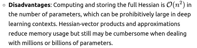
What are the key differences between first-order and second-order optimization methods, and when might we prefer one over the other?
First-order methods like standard (S)GD and its variants use only gradient information. They tend to be simpler to implement and computationally cheaper per iteration, especially for high-dimensional problems. They do, however, often require fine-tuning of learning rates and can converge slowly in ill-conditioned optimization landscapes.
Second-order methods (e.g., Newton’s Method, quasi-Newton methods like L-BFGS) use gradient and Hessian (or approximate Hessian) information. The Hessian matrix captures curvature, allowing for potentially more direct paths to minima:
Advantages: They can converge in fewer iterations and handle ill-conditioning better because they adapt the step direction and step size via curvature.

When to Prefer One or the Other:
High-Dimensional Neural Networks: First-order methods are standard because second-order methods require enormous computational resources.
Smaller or Medium-Sized Problems: Quasi-Newton methods can yield faster convergence and better hyperparameter robustness.
Ill-Conditioned but Manageable Dimensionality: Second-order approximations excel, especially if the Hessian can be efficiently approximated.
In practice, for large-scale machine learning, first-order methods augmented with adaptive learning rates (Adam, RMSProp) are overwhelmingly the default, whereas second-order methods might be used in smaller data and lower-dimensional optimization tasks for faster convergence.
How does gradient descent handle asynchronous or distributed training scenarios?
In large-scale machine learning, it’s common to distribute training across multiple machines or GPUs. There are two broad strategies:
Synchronous Training:
Each worker (GPU/machine) computes gradients on its mini-batch.
Gradients are averaged (or summed) across workers.
Parameters are updated globally only after all workers finish a “round.”
Pros: Convergence is more predictable because each update sees consistent, aggregated gradient information.
Cons: If one worker is slow (straggler), all others must wait, creating potential inefficiencies.
Asynchronous Training:
Each worker calculates gradients and updates parameters independently, using a shared parameter server or distributed storage.
Workers do not necessarily wait for others; they push updates as soon as they compute them.
Pros: Potentially faster throughput since there’s no waiting for slow workers.
Cons: The parameter updates might become stale because multiple workers may be updating simultaneously with different old parameter states. This can slow or disrupt convergence.
Pitfalls:
Learning Rate Management: Adjusting the learning rate becomes more nuanced. Large-scale setups with many workers need smaller per-worker learning rates or specialized algorithms to avoid blowing up the loss.
Communication Overhead: Sharing gradients or parameters continuously can bottleneck distributed systems.
Stale Gradients: Asynchronous updates use outdated model parameters when computing new gradients. Techniques like bounded staleness or flexible consistency levels can mitigate this effect.
Despite these challenges, distributed gradient descent, particularly synchronous mini-batch approaches, remains the standard for training massive deep networks in industry-scale environments (e.g., large language models, image recognition tasks).
How can we accelerate convergence with momentum or related techniques?
Momentum-based optimizers aim to simulate a physical “momentum” term, helping the optimization move consistently in beneficial directions and dampen oscillations in orthogonal directions.
Vanilla Momentum:
Maintains a velocity vector (an exponential moving average of past gradients).
Updates incorporate both the current gradient and the previous velocity, effectively smoothing the trajectory.
Typical update rule:

Hyperparameter β (momentum decay) controls how strongly past gradients influence the current update.
Nesterov Accelerated Gradient (NAG):
Predicts the next step before computing the gradient, offering a more precise correction:

Often converges faster in practice than vanilla momentum.
Potential Pitfalls:
If β is too high, the updates can overshoot minima due to excessive inertia.
Momentum can magnify parameter updates if the learning rate is not tuned alongside β.
In non-convex settings, momentum can sometimes skip over narrow but deep minima.
Despite these pitfalls, momentum-based methods (including Adam, RMSProp, and others that combine momentum with adaptive learning rates) are the default for training deep neural networks because they generally reduce training time and improve convergence consistency.
How do we detect and handle exploding or vanishing gradients in deep networks?
Deep neural networks often experience gradient magnitudes that are either excessively large (exploding) or extremely small (vanishing), especially when dealing with recurrent networks or very deep architectures.
Vanishing Gradients:
Occur when gradient propagation through many layers diminishes to near zero, halting effective learning in early layers.
Common solutions include:
Activation Functions like ReLU or variants that avoid saturation.
Initialization Schemes (He initialization, Xavier initialization) designed to maintain variance across layers.
Batch Normalization or Layer Normalization to stabilize gradient flows.
Exploding Gradients:
Occur when gradients accumulate excessively, causing large parameter updates and possible numerical instability.
Common remedies include:
Gradient Clipping: Rescale gradients if their norm exceeds a specified threshold.
Adjusting Network Architecture: Simplifying or carefully designing architectures to avoid extremely large weight matrices.
Learning Rate Reduction: Sometimes lowering the learning rate is enough to manage moderate explosions.
Practical Pitfalls:
Overly aggressive gradient clipping can hamper the optimization if it’s triggered too often.
Even when vanishing or exploding gradients are mitigated, suboptimal initialization can prolong training.
Some architectures (e.g., LSTM, GRU in RNNs) are explicitly designed to reduce vanishing gradients but can still face exploding gradients for very long sequences.
How do we ensure fair updates when the dataset has imbalanced classes or widely varying feature scales?
Imbalanced Classes:
If one class greatly outnumbers others, stochastic gradient updates tend to reflect mostly the dominant class, potentially ignoring minority classes.
Solutions include:
Oversampling / Undersampling: Adjusting the dataset distribution or using synthetic data (SMOTE for example).
Weighted Loss Functions: Multiply the loss by class-specific weights, so the minority class exerts a proportionally larger influence on the gradient.
Sampling Strategy: Stochastically pick data from classes with appropriate frequencies to balance out the updates.
Varying Feature Scales:
Large-scale features might dominate the gradient, overshadowing smaller-scale features.
Solutions include:
Feature Normalization: Standardizing or normalizing each feature to have comparable magnitude.
Adaptive Optimizers: Methods like Adam or Adagrad naturally adjust per-parameter updates based on past gradient magnitudes.
Common Pitfalls:
Overfitting to minority classes if oversampling is excessive.
Potential numeric instability if feature scaling is done inconsistently (e.g., partial standardization).
Weighted losses can become tricky to tune manually; an imbalanced dataset might still show misleading accuracy metrics, so deeper evaluation (precision, recall, F1 scores) is crucial to confirm that the model is improving properly for minority classes.
How do different data preprocessing steps, like normalization or dimensionality reduction, affect gradient descent?
Normalization:
Scaling input features to a common range or distribution often yields more stable and quicker convergence. It prevents any single dimension from dominating the gradient.
When input distributions shift dramatically, gradients become skewed, risking slow or divergent training.
Dimensionality Reduction:
Techniques like PCA or autoencoders can condense high-dimensional data into fewer features, potentially simplifying the optimization landscape.
If relevant information is lost during dimensionality reduction, the model might underperform or converge to a suboptimal region.
Potential Edge Cases:
Online Updates vs. Offline Scaling: If data is arriving in streaming fashion, you must update normalization statistics adaptively to maintain correct data scale estimates.
Over-normalization: In some tasks, data with constant or near-constant scaled values can hamper the model’s ability to learn significant distinctions.
Dependency on the Model Architecture: Some architectures might learn scale invariance themselves (e.g., through learned normalization layers), so external normalization is less critical but still beneficial for stability.
Effective preprocessing often forms the foundation of robust gradient-based optimization. Even advanced optimizers can struggle if the raw data is not scaled sensibly.
How do we properly evaluate convergence during iterative gradient-based training?
Loss Monitoring:
Track the training loss and possibly a validation loss over iterations or epochs. A plateau or minimal change over several iterations suggests convergence.
A sudden drop or spike can indicate numerical issues, a poor learning rate, or data irregularities.
Gradient Norm:
Evaluate the norm of the gradients. If gradients become consistently small, the parameters might be near a stationary point.
However, a small gradient does not guarantee a global minimum—this can also happen at saddle points.
Early Stopping:
Stop training if validation performance has not improved for a certain number of epochs. This prevents overfitting and also signals that further gradient updates yield diminishing returns.
Practical Pitfalls:
Loss can flatten and appear “converged” while the model continues to improve slowly on more subtle metrics (for example, exact top-1 accuracy in classification tasks).
Validation loss might diverge from training loss if overfitting begins. Strict reliance on training metrics can be misleading.
In large-scale deep learning, the objective might not strictly converge to a single global optimum, but a near-minimum region. The user must balance more training time against diminishing improvements.
When evaluating convergence, it’s crucial to look at multiple signals (training loss, validation loss, accuracy, gradient norms, etc.) and adapt training strategies—like adjusting the learning rate or momentum—if progress stalls unexpectedly.