
ML Interview Q Series: Explain how the kernel trick operates in SVMs, illustrate with a straightforward example, and discuss your approach for determining which kernel function to use

📚 Browse the full ML Interview series here.
Short Compact solution
When selecting a kernel, one can opt for linear kernels when the data appears linearly separable or can be better modeled by simpler linear decision boundaries, and pick nonlinear kernels like the Radial Basis Function (RBF) or polynomial kernels when the data is complex and likely not linearly separable. Domain knowledge can guide kernel selection, or one can rely on systematic hyperparameter searches (like grid search) that compare candidate kernels using relevant performance metrics such as accuracy, F1, or AUC.
Comprehensive Explanation
Definition of the Kernel Trick
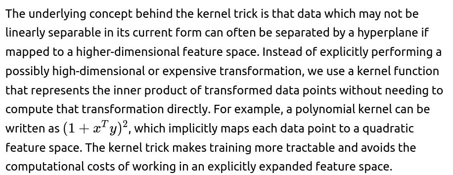
The kernel trick is a strategy that lets Support Vector Machines (SVMs) or other kernel-based methods effectively operate in a higher-dimensional feature space without ever computing coordinates of data in that space. Instead, the SVM only needs the dot products of pairs of transformed points. This dot product in the high-dimensional space is encapsulated by a kernel function. Formally:
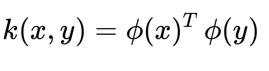
The function k is the kernel, and ϕ(⋅) is an implicit mapping from the original input space to a (potentially very high) dimensional feature space.
Example: Polynomial Kernel

In practice, domain expertise can help identify which kernel is more suitable. If no domain insights are available, cross-validation and hyperparameter search can help select among candidate kernels based on metrics like accuracy, F1-score, AUC, or any other measure important in the domain.
Implementation Considerations
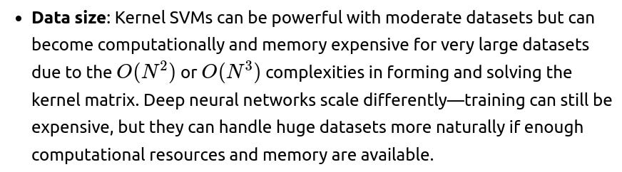
When training an SVM, the main computational bottleneck is constructing and storing the kernel matrix and then solving the corresponding optimization problem. For large datasets, kernel-based methods can be memory-intensive because they typically require a matrix with dimensions proportional to the number of training samples squared. Approximation strategies such as randomized feature maps or specialized training algorithms can alleviate these issues.
Pitfalls and Challenges
If the kernel parameters are not selected properly, the model can overfit or underfit. For instance, an RBF kernel’s gamma parameter controls how much influence each training instance has; too large a gamma can cause overfitting, while too small can lead to underfitting. Overly high polynomial degrees can also cause extreme complexity, leading to overfitting. Proper normalization and scaling of features are often important to make the kernel function behave consistently across different feature dimensions.
Follow-up question: Could you explain how one might perform a systematic search for the best kernel and kernel hyperparameters in an SVM?
A common approach is to use cross-validation to evaluate a grid or random search over candidate kernel types (linear, polynomial, RBF, and so on) and their hyperparameters. For a polynomial kernel, one might vary the degree and coefficient in the polynomial. For an RBF kernel, one might vary parameters such as gamma. The process involves defining a range of possible values for each hyperparameter, training and validating on different data folds, and then identifying the kernel and hyperparameter combination that optimizes a chosen performance metric. More advanced approaches like Bayesian optimization can also be used to more efficiently explore hyperparameter space.
Follow-up question: Why not always use a higher-dimensional kernel, like a very high-degree polynomial kernel, to guarantee that the data becomes separable?
Very high-degree polynomial kernels can indeed create extremely flexible decision boundaries but tend to risk overfitting, where the model fits the training data well but fails to generalize to unseen data. This risk grows if the dataset is limited in size or if feature noise is present. Moreover, higher-degree kernels typically include many interaction terms, complicating training and increasing the chances of numerical instability. Balancing model capacity and regularization through parameter tuning is essential to maintaining good generalization.
Follow-up question: In practice, how do you deal with very large datasets when using kernel SVMs?
For very large datasets, the cost of computing and storing the full kernel matrix becomes prohibitive, since the matrix size grows as the square of the number of samples. One strategy is to use approximate kernel methods that map data into an explicit but lower-dimensional feature space, for example using Random Fourier Features for RBF kernels. Another strategy is to adopt specialized large-scale solvers or online algorithms that handle data in smaller batches. In addition, linear SVMs are often preferred if one can demonstrate that a nonlinear separation is not strictly necessary.
Below are additional follow-up questions
1) How can we interpret decision boundaries from a kernel SVM model, and what challenges might arise?
Interpretation of a kernel SVM’s decision boundary can be less straightforward than that of a linear SVM or simpler classifiers. This is because the boundary is determined by inner products in a high-dimensional feature space, making it more difficult to visualize or explain in the original input space. One common approach to gain some insight is to analyze which support vectors are most influential. By understanding which data points end up as support vectors and how the kernel function measures their similarity to other points, you can gauge why a particular classification boundary was drawn.
Potential pitfalls include:
High-dimensional complexity: If you’re using complex kernels (e.g., higher-degree polynomial or RBF), the boundary can have highly non-linear shapes, making it opaque to simple, intuitive explanations.
Misleading visualizations: Visualizing in 2D or 3D for interpretability can mask the complexity if your data naturally spans many dimensions.
Overfitting: Highly flexible kernels can create very intricate boundaries that are hard to interpret and may overfit.
2) Is the kernel trick guaranteed to yield a valid kernel for any arbitrary function we pick, and how do we verify that a kernel is valid?
Not every function qualifies as a valid kernel. A valid kernel must satisfy the properties required by Mercer’s theorem, specifically that the kernel matrix it produces must be symmetric and positive semi-definite for any set of data points. If it fails these conditions, the SVM’s quadratic optimization can become infeasible or yield nonsensical solutions.
Verifying a kernel’s validity can be done by:
Checking positive semi-definiteness: For any finite collection of input points, the kernel matrix (the Gram matrix) must have no negative eigenvalues. This can be tested, though it can be expensive for large datasets.

3) How do we handle multi-class classification with kernel SVMs?
Although the basic SVM formulation is inherently binary, one can extend it to multi-class settings using standard strategies such as:
One-vs-Rest (OvR): Train one SVM for each class to separate that class from all remaining classes. In inference, pick the class whose SVM has the highest decision function value.
One-vs-One (OvO): Train an SVM for every pair of classes. With N classes, there will be N(N−1)/2 binary classifiers. In inference, use a voting or max-wins scheme across these pairwise classifiers.
Pitfalls include:
Increased computational cost: With OvO, you train a large number of binary classifiers if the number of classes is large.
Inconsistent boundaries: Each pairwise classifier might learn a boundary that doesn’t necessarily align with other pairwise boundaries for different class pairs, sometimes leading to ambiguous predictions if the data is especially complex or noisy.

4) If your features differ widely in scale, how does this impact the kernel SVM, and how should you address it?
SVMs are very sensitive to feature scales, especially with certain kernels like RBF. If one feature has a much larger numeric range than others, its distance-based impact in the kernel function might dominate, leading to poorly shaped decision boundaries or suboptimal margin placement.
To mitigate this:
Feature scaling (e.g., standardization to zero mean and unit variance or min-max normalization) before training is highly recommended.
Cross-validation should be done on data that is scaled using parameters (mean, standard deviation, etc.) fit only on the training set of each fold, to avoid data leakage.
Pitfalls:
Data leakage: Failing to apply scaling correctly at each step can leak information from the validation set into your model training.
Overfitting or underfitting: Using improper scales or incorrectly selecting scaling parameters may lead to suboptimal performance.
5) How do kernel SVMs handle noise or outliers in the training data, and what parameters control that behavior?
Outliers and noisy points can heavily influence the decision boundary if you do not add proper regularization. In soft-margin SVMs, the C parameter controls the trade-off between maximizing the margin and minimizing classification errors on the training data.
Large C: The SVM places a high penalty on misclassifying points, potentially warping the boundary to correctly classify every outlier. This can reduce margin size and increase overfitting.
Small C: Allows more slack for misclassifying certain points or placing them within the margin, typically leading to a smoother boundary but possibly underfitting.
In kernel SVMs, kernel parameters also affect sensitivity to outliers. For instance, in the RBF kernel, gamma controls the locality of the radial function. A very large gamma can cause the SVM to pay excessive attention to each point, increasing overfitting risk.
6) What are some real-world considerations when deciding between a kernel SVM and a deep neural network for complex classification tasks?
Feature engineering: Kernel SVMs rely on choosing or engineering a suitable kernel, while deep networks can learn hierarchical representations automatically if enough data and computational resources exist.
Interpretability: Both kernel SVMs and neural nets can be black-box models, but local interpretability might be somewhat more intuitive in SVMs by analyzing support vectors, whereas deep nets typically require specialized interpretability techniques (like saliency maps, layer-wise relevance propagation, etc.).
Hardware constraints: Training advanced neural networks may require specialized GPU or TPU hardware. Kernel SVMs can run on CPUs, although as the dataset grows, memory constraints for the kernel matrix might still be a bottleneck.
Pitfalls:
Underutilizing data: If you have massive datasets without an effective kernel approximation, SVMs might be infeasible.
Architecture choices: In neural networks, a poor choice of architecture or hyperparameters can yield subpar results, just as a poor kernel choice can harm SVM performance.
7) How might you decide between a polynomial kernel and an RBF kernel in practice, and what are the trade-offs?
Polynomial kernel: Good if you suspect polynomial-like feature interactions or if the data is structured in a way that polynomial terms are naturally meaningful (e.g., interactions up to some degree). However, a high-degree polynomial might cause overfitting and can grow very large in dimensionality.
RBF (Gaussian) kernel: Often considered a “universal approximator,” capable of fitting highly non-linear boundaries. It relies heavily on the gamma parameter. With a well-chosen gamma, it can handle diverse shapes in the data distribution.
Trade-offs:
Interpretability: Polynomial kernels can sometimes be easier to interpret if the polynomial degree is small. RBF kernels are more difficult to interpret directly.
Parameter sensitivity: The RBF kernel requires tuning gamma and C, while a polynomial kernel has parameters for degree, possibly a constant term, and the regularization parameter C. Both can be tuned via cross-validation.
8) How does the number of support vectors scale with kernel choice, and why does it matter?
Depending on the kernel and data complexity, the number of support vectors might grow significantly. A more flexible kernel (like an RBF) can cause many points to lie near the decision boundary, increasing the number of support vectors. Having too many support vectors:
Increases inference cost: Each prediction requires computing the sum of kernel functions between the test point and each support vector. With large support sets, this can slow down prediction.
Indicates potential overfitting: If a large fraction of the training set becomes support vectors, the model might be memorizing training examples rather than capturing a generalizable pattern.
Pitfalls:
Memory constraints: Storing a large set of support vectors can consume significant memory, especially for large-scale problems.
Model interpretability: A huge number of support vectors can be unwieldy for understanding why the SVM made particular decisions.
9) What if the dataset includes a large number of categorical features — can we still apply kernel SVMs effectively?
Applying kernel SVMs directly to many high-cardinality categorical features can be problematic because naive encodings (such as one-hot encoding) can explode dimensionality, making the kernel matrix massive. Potential solutions include:
Embedding or hashing: Use an embedding or a hashing trick to reduce dimensionality.
Domain-specific encoding: If you have domain knowledge, you might encode categories in ways that preserve meaningful relationships, then apply the kernel on top of these numerical embeddings.
Pitfalls:
Loss of interpretability: Compressed or hashed representations can obscure which specific categories contribute to decisions.
Data sparsity: One-hot vectors can be extremely sparse, leading to extremely sparse kernel matrices that might not be as beneficial for certain kernel methods unless carefully handled.
10) How can you mitigate numerical stability issues in kernel SVMs, especially for large datasets or high-dimensional data?
Numerical instability can appear in various ways, such as kernel matrix entries becoming too large or too small (underflow / overflow). Strategies to mitigate this include:
Regularization parameters: Careful tuning of C and any kernel-specific parameters helps ensure that the optimization problem remains well-conditioned.
Feature scaling or normalization: Keeping features on a comparable scale can prevent large differences in magnitude from causing excessively large entries in the kernel matrix.
Approximation techniques: Instead of forming the full kernel matrix, use approximate methods (e.g., random Fourier features for the RBF kernel). These typically result in lower memory usage and can improve numerical stability in some cases.
Software and libraries: Choosing reliable numerical linear algebra libraries (e.g., those that handle rank-deficient or near-singular matrices gracefully) can reduce floating-point issues.
Pitfalls:
Floating-point precision: When data or kernel parameters lead to extremely large or tiny values, standard double-precision arithmetic might not be sufficient to maintain stability.
Ill-conditioning: If the kernel matrix is close to singular, small changes in the data or parameters can drastically change the solution.