
ML Interview Q Series: Explain how the “Greedy Splitting” method is applied when building a Decision Tree


📚 Browse the full ML Interview series here.
Comprehensive Explanation
Greedy splitting in a decision tree refers to the procedure of choosing a single split at each internal node, with the objective of locally optimizing a certain metric (for example, information gain or Gini impurity) without exploring the long-term consequences of that choice. Essentially, at each node, the split that appears best at that moment is chosen. This method is computationally efficient, but it does not necessarily guarantee a globally optimal solution for the entire tree.
A typical example is the use of the entropy-based criterion in classification tasks. Entropy measures the homogeneity of a set of examples. When we perform a split on a feature, we want to reduce the entropy as much as possible to create more “pure” subsets. Alternatively, Gini impurity is often used in modern implementations like the CART algorithm.
Below is one common formulation for entropy-based information gain, a key concept in many decision tree algorithms when considering a classification scenario:
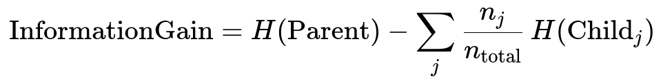
Where:
H(Parent) is the entropy of the parent node.
Child_j is the jth child node after the split.
n_{j} is the number of samples going to Child_j.
n_{total} is the total number of samples in the parent node.
H(Child_j) is the entropy of that jth child node.
In many algorithms, we systematically evaluate every feature and every possible way of splitting that feature to determine which split yields the largest reduction in impurity (or the largest gain in purity). Because the search is done only at the node level—without looking ahead to possible future splits—it is a greedy approach. Once this split is chosen, the procedure is repeated recursively for the new subtrees, continually partitioning until some stopping criterion is met (e.g., maximum tree depth, minimum node samples, or purity thresholds).
Greedy splitting ensures efficiency, since exploring all possible combinations of splits at multiple levels would be computationally prohibitive. However, it may lead to suboptimal overall tree structure if an early split is not aligned with an optimal partitioning at lower levels in the tree.
Below is a simple Python snippet illustrating the general idea of checking a possible split using Gini impurity (though the code is quite simplified and does not represent a fully optimized implementation):
import numpy as np

def gini_impurity(labels):
    """
    Compute Gini impurity for a list/array of class labels.
    """
    unique_classes, counts = np.unique(labels, return_counts=True)
    probabilities = counts / counts.sum()
    return 1.0 - np.sum(probabilities**2)

def best_split(X, y):
    """
    Find the best split among all features for a single node.
    X is feature matrix, y is labels.
    """
    best_feature_index = None
    best_threshold = None
    best_impurity = float('inf')

    current_impurity = gini_impurity(y)

    for feature_idx in range(X.shape[1]):
        # Potential thresholds: unique values of the feature
        feature_values = np.unique(X[:, feature_idx])
        for threshold in feature_values:
            # Split the data
            left_indices = X[:, feature_idx] <= threshold
            right_indices = X[:, feature_idx] > threshold

            left_labels = y[left_indices]
            right_labels = y[right_indices]

            # Weighted average Gini
            left_impurity = gini_impurity(left_labels)
            right_impurity = gini_impurity(right_labels)
            w_left = len(left_labels) / len(y)
            w_right = len(right_labels) / len(y)
            weighted_impurity = w_left * left_impurity + w_right * right_impurity

            # Compare if this split is better
            if weighted_impurity < best_impurity:
                best_impurity = weighted_impurity
                best_feature_index = feature_idx
                best_threshold = threshold

    return best_feature_index, best_threshold, current_impurity - best_impurity
This piece of code calculates Gini impurity at a node and evaluates each possible threshold for every feature, then picks whichever yields the largest reduction in impurity. This local, or “greedy,” selection repeats at every node.
How Greedy Splitting Happens in Practice
For classification trees:
At each node, a splitting criterion such as information gain or Gini impurity is computed for all possible partitions.
The algorithm chooses the split that yields the best improvement in that metric.
The resulting subsets form new child nodes, and the procedure continues recursively.
For regression trees:
The impurity measure can be something like the variance of the target values at each node.
Splitting is chosen to minimize the sum of squared deviations within the child nodes.
This process is repeated until certain stopping criteria are met, like reaching a specified tree depth or having too few samples in a leaf node to continue splitting effectively.
Potential Drawbacks of Greedy Splitting
The principal criticism is that it does not look at the longer-term effect of a split. For instance, a locally suboptimal split might in certain cases enable an excellent partition at lower levels, producing better global performance. Nonetheless, exploring all possible combinations to find the truly best sequence of splits is computationally expensive, making greedy splitting a reasonable trade-off for many real-world applications.
Possible Follow-Up Questions
Can the Greedy Splitting Procedure Miss the Globally Optimal Tree?
Yes, because it does not backtrack or look ahead. Each choice is based solely on immediate gain rather than potential downstream improvements. Decision trees do not typically guarantee a global optimum under this splitting strategy.
How Do You Choose Between Different Impurity Metrics?
Common options include Gini impurity and entropy-based information gain for classification tasks. Gini impurity tends to be faster to compute. Empirically, both tend to produce similar results, although Gini sometimes favors splits that isolate the most frequent class. The best choice can depend on the specific dataset and performance requirements.
Could Using Greedy Splitting Lead to Overfitting?
Yes. Because decision trees continue branching until they reach a pure leaf or a stopping criterion, the tree can become overly complex and perfectly classify the training data, failing to generalize well. Techniques like pruning (post-pruning or pre-pruning) mitigate this problem by limiting the tree’s growth or cutting back branches that do not contribute to improving validation performance.
Are There Any Extensions That Look Beyond a Single Greedy Split?
Yes, there are algorithms that attempt more global optimization, like “best-first” tree growth or lookahead strategies. These, however, can be significantly more computationally expensive and thus are less common in practice. Ensembles like Random Forests or Gradient Boosted Trees leverage the idea of building many trees or sequentially refined trees, sometimes improving performance without explicitly performing global optimization in a single tree.
Are There Situations Where Greedy Splitting Is Still Quite Effective?
Yes, in many real-world tasks, especially those with a large feature space and large sample sizes. The simplicity of the greedy split approach often yields highly interpretable trees, and with proper regularization (like pruning), it can handle complex tasks well. The speed of training and the relatively small memory footprint are additional advantages for large datasets.