
ML Interview Q Series: Explain the key advantages of adopting a dynamic pricing approach, and discuss how you might determine both supply and demand in this scenario.

📚 Browse the full ML Interview series here.
Comprehensive Explanation
Dynamic pricing refers to adjusting the cost of products or services in near-real time based on various market factors. This strategy relies heavily on understanding how supply and demand shift over time and under different conditions. Below is a deep dive into its benefits, followed by ways to estimate supply and demand and the statistical or machine learning approaches that support it.
Benefits of Dynamic Pricing
One major advantage is revenue maximization. By raising prices when demand spikes (such as holidays or limited availability) and lowering them during slower periods, a company can capture different consumer willingness to pay. This also helps with inventory management: when stock levels are high, lowering the price can stimulate demand, whereas constrained inventory might warrant raising the price.
It also provides a competitive edge, especially in industries where competitors frequently change their prices (e.g., airlines, ride-sharing). Companies that effectively manage dynamic pricing can stay aligned with evolving market conditions and quickly respond to external shifts—like a sudden competitor discount or a sudden surge in raw material costs.
Additionally, it offers personalized pricing opportunities. Modern algorithms can factor in customers’ browsing and purchasing history, location, and other data points to refine price recommendations. This creates a scenario in which each consumer pays a price that better reflects their own demand curve.
Estimating Supply and Demand
Demand and supply can be viewed as functions that change with price and other variables such as seasonality, marketing activities, and macroeconomic indicators. In classical economic theory, you might see them modeled as something akin to:

where:
Q_{d} in text means the demanded quantity.
a in text means the intercept (base level of demand if price = 0).
b in text means the slope (how much demand falls when price increases).
P in text means the price.
where:
Q_{s} in text means the supplied quantity.
c in text means the base level of supply if price = 0.
d in text means how supply changes with respect to price.
The actual demand and supply curves in real-world settings can be more complex. Firms typically estimate them using data-driven approaches, such as regression analysis or time series forecasting. The strategy involves collecting historical data on pricing, quantity sold, marketing expenditures, competitor activities, seasonality metrics, and external economic factors. Machine learning models (e.g., gradient boosting or neural networks) help capture complex relationships and interactions in that data.
Example: Simple Demand Curve Estimation
Below is a simple snippet showing how one might estimate a basic demand curve from data using Python’s statsmodels or sklearn libraries. This snippet is purely illustrative and omits many real-world complexities (e.g., supply constraints, competitor effects).
import pandas as pd
import numpy as np
from sklearn.linear_model import LinearRegression

# Suppose you have a DataFrame with columns: 'price' and 'units_sold'
data = pd.DataFrame({
    'price': [10, 12, 14, 16, 18, 20],
    'units_sold': [1000, 850, 720, 600, 500, 400]
})

X = data[['price']]
y = data['units_sold']

# Fit a simple linear regression
model = LinearRegression()
model.fit(X, y)

# Model coefficients
b = model.coef_[0]
a = model.intercept_

# Predict demand for a given price
sample_price = 15
predicted_demand = model.predict([[sample_price]])

print(f"Demand Equation: Q = {a:.2f} - {abs(b):.2f} * P")
print(f"Predicted demand for price ${sample_price} is {predicted_demand[0]:.2f} units")
In more advanced implementations, you would employ time series modeling to capture seasonality or ARIMA-like patterns, and you might use feature engineering to represent external factors such as competitor pricing or marketing initiatives.
Price Elasticity of Demand
Another crucial aspect is elasticity: how sensitive demand is to changes in price. A common elasticity formula is shown below:
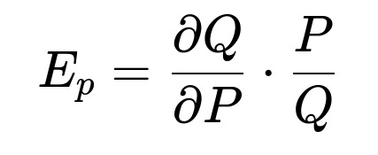
where:
E_{p} in text means price elasticity of demand.
Q in text means the quantity demanded.
P in text means the price.
If E_{p} in text is less than -1 (in absolute value), the product is price elastic, meaning a small price change leads to a more-than-proportional change in demand. This information helps you decide whether you can freely raise prices or if doing so might drop demand too much.
Follow-Up Questions
How can you account for external factors, like competitor pricing or marketing campaigns, in dynamic pricing?
One effective approach is to add more features into the regression or machine learning model that reflect these external influences. This might include historical competitor prices (lagged by days or weeks), competitor promotions, or marketing spending data. You can use distributed lag models or time series methods to capture delayed effects of these variables on your own demand. Adding these variables can help you see whether your sales volume is influenced by competitor undercutting, new product launches, or advertising surges.
You can also explore specialized models such as Vector Autoregression, which simultaneously captures how multiple time series (e.g., your sales, competitor’s pricing, marketing campaigns) influence each other. This enables a more holistic view of the market dynamics.
What challenges arise in implementing a dynamic pricing system in production?
Practical hurdles include data latency and reliability. If your system is designed to update prices hourly, you need accurate, near-real-time data on sales, inventory, competitor behavior, and market signals. Another concern is the possibility of price wars. If several companies use automated dynamic pricing solutions, they might continuously undercut each other, ultimately harming profits and brand perception.
There are also user experience and fairness concerns, especially in industries like ride-sharing. Rapidly fluctuating prices can cause negative public perception if users feel they are being exploited. Regulatory considerations might also exist in certain markets, where price discrimination or predatory pricing practices are scrutinized.
In dynamic pricing, how do you prevent overfitting to historical demand patterns?
Using techniques such as regularization (e.g., Ridge or Lasso in regression) or cross-validation is crucial. Historical relationships might not hold in future scenarios. Partitioning your dataset into training and validation sets and ensuring your model generalizes well under different conditions reduces overfitting risks.
You can also maintain a small but continuous exploration strategy—periodically offering random price variations to gather fresh data about new demand patterns. This helps the model adapt to shifting customer behaviors or external conditions (e.g., new competitor entering the market). Bayesian approaches can also allow for uncertainty estimation, giving you a measure of confidence in the model’s predictions.
How can seasonality or special events be incorporated into forecasting?
Seasonality can be captured with time series decomposition, Fourier transforms, or dummy variables representing periods like weekends, holidays, or significant cultural or sporting events. For instance, if the demand for an item spikes before major festivities, you can add a feature that indicates the days or weeks leading up to the holiday. This feature helps your model anticipate the surge in demand.
In deep learning approaches (e.g., sequence models like LSTM networks), seasonality can be learned implicitly if sufficient historical data is provided. But it’s still good practice to create explicit features for known seasonal or cyclical patterns.
How does the concept of supply constraints or capacity limits factor into dynamic pricing decisions?
If the supply of the product is limited, the model can incorporate constraints to prevent prices from dropping too low when remaining inventory is scarce. One might include an optimization layer that attempts to maximize revenue subject to constraints on available inventory.
If there is a production capacity that can ramp up, you might have a partial dependence on price. When you see demand rising, you can increase the price to slow sales while your capacity catches up. This is especially common in on-demand services or perishable inventory scenarios (like hotel rooms or airline seats). Incorporating supply constraints ensures that your pricing engine does not inadvertently sell more inventory than you can fulfill or create dissatisfied customers by overselling.
Could you discuss the role of reinforcement learning in dynamic pricing?
Reinforcement learning (RL) can adapt pricing policies based on reward signals such as revenue or profit. The RL agent learns through trial and error, exploring price variations and observing their effects on demand. Over time, it refines a policy that yields optimal or near-optimal returns, given the constraints.
Challenges in RL-based pricing include ensuring sufficient exploration—particularly in high-dimensional price spaces—and avoiding abrupt price changes that alienate customers. You also need robust demand simulations or large volumes of real-time transactional data for the RL agent to learn effectively.
Is there a risk of collusion if competitors also use dynamic pricing algorithms?
Yes, this is a regulatory concern in some jurisdictions. If multiple market players are using sophisticated algorithms, there could be an emergent phenomenon resembling collusion. The algorithms might learn to maintain higher prices rather than competing aggressively, which can draw scrutiny from regulators. Ensuring transparency in how your pricing engine arrives at decisions and including policy-based constraints can help mitigate these risks.
Below are additional follow-up questions
How do you handle real-time data latency in a dynamic pricing system, and what strategies can mitigate issues from delayed or incomplete information?
Data latency occurs when there is a delay between collecting information (e.g., current demand, inventory levels, competitor moves) and feeding it into the pricing algorithm. This can lead to outdated signals influencing price updates, which results in suboptimal or even conflicting decisions. One strategy is to implement a near-real-time data pipeline using streaming technologies (such as Apache Kafka or AWS Kinesis) so that every demand signal is quickly ingested and integrated into the pricing engine. Another approach is to estimate short-term future states of demand through predictive models, effectively bridging the gap until actual data arrives.
A further mitigation technique involves designing robust fallback rules for interim periods when data is missing or outdated—such as having default price floors/ceilings or reverting to the last stable price. Bayesian updates can also be employed to maintain a distribution over possible demand states, allowing partial updates even when only partial data is available.
Potential pitfalls arise if you do not account for uneven data availability across different geographical markets or product lines. One region might have real-time data pipelines in place, while another still relies on batch updates. This discrepancy can create uncoordinated pricing decisions and harm brand consistency. Monitoring data completeness and reliability metrics is essential to detect such issues early.
In what ways can you measure the success of a dynamic pricing system beyond short-term revenue increases?
Revenue, while critical, is not always the sole indicator of a successful dynamic pricing strategy. Additional metrics include customer lifetime value (CLV), user acquisition or retention rates, and brand perception. By tracking repeat purchases or average purchase frequency, you detect whether customers are reacting negatively to perceived price volatility. Tracking net promoter score (NPS) can also highlight potential damage to brand reputation if people feel prices are unfair.
Measuring inventory turnover is another valuable indicator. Faster turnover at consistent or higher profit margins suggests the pricing system is effectively balancing supply and demand. Conversely, if the inventory stagnates despite price adjustments, there might be an overestimation of demand or poor elasticity modeling. Monitoring cart abandonment rates for e-commerce sites is also insightful, as dynamic prices that shift too aggressively could push users to abandon their purchase.
One subtle pitfall is ignoring long-term cannibalization. If raising prices temporarily boosts revenue but drives away customers in the long run, the dynamic pricing strategy is self-defeating. Hence, combining short-term revenue metrics with multi-period models of customer value and brand loyalty is crucial.
Could you explain how multi-armed bandit approaches might be useful for dynamic pricing, and how they compare to standard machine learning methods?
Multi-armed bandit techniques allow you to explore multiple pricing “arms” (i.e., price points or pricing strategies) while exploiting the best-known option at any given time to maximize cumulative reward. This is particularly powerful when you do not have a large historical dataset or when you are dealing with rapidly changing conditions. The bandit algorithm continuously updates its understanding of which price yields the highest reward (e.g., expected revenue or profit) given current market conditions.
Unlike classical regression or supervised learning approaches, multi-armed bandit algorithms can adapt more quickly when a sudden shift in user behavior occurs, as they maintain an active exploration strategy. However, pure bandit methods might struggle to incorporate complex contextual factors (like competitor pricing or marketing spend) unless you use contextual bandit extensions. In these extensions, additional features (e.g., user segment, time of day) refine the selection of which “arm” (price point) is optimal.
A potential edge case arises when the action space (number of possible prices) is very large. If you have a wide range of possible price points, a naive bandit approach may not converge efficiently, as it will take a long time to explore them all. This is often mitigated by discretizing possible prices or by leveraging parametric or semi-parametric bandit models that exploit structure in the pricing function.
How do you plan for black swan events or extraordinary disruptions that drastically alter demand or supply?
Black swan events—like natural disasters, pandemics, or sudden regulatory changes—can upend historical demand patterns and leave existing models almost useless. One mitigation strategy is to maintain contingency-based models that can be rapidly retrained or overridden by rule-based heuristics when outlier conditions are detected. Using anomaly detection methods in your time series or transaction logs can automatically flag periods of unusual activity, triggering a mode switch in the pricing algorithm.
Stress testing is another valuable technique. You can simulate extreme scenarios—like a 90% drop in demand—to see how the dynamic pricing system responds. Identifying how the pricing logic behaves under these simulations reveals vulnerabilities, such as overshooting price reductions or drastically overpricing items in a panic-driven market. Another subtle issue is supply chain constraints; if you rely on just-in-time inventory management, a shock could suddenly make you unable to fulfill demand. In this scenario, you might employ a safeguard to freeze or raise prices gradually to preserve inventory for essential customers or ensure fair distribution.
How do data privacy concerns affect personalized dynamic pricing, and what are best practices to ensure compliance and fairness?
Personalized dynamic pricing often involves collecting user data, such as purchase history, browsing behavior, or geolocation. Data privacy regulations (e.g., GDPR in the EU, CCPA in California) impose limits on how you collect, process, and store personally identifiable information (PII). A best practice is to anonymize or pseudonymize user information, storing only aggregated metrics or using unique identifiers that cannot be traced to an individual directly. Regular audits of data collection pipelines help ensure there are no hidden leaks of PII.
Fairness issues arise if certain demographic groups face systematically higher prices. To address these concerns, you can implement fairness constraints in your algorithms, effectively bounding the allowable difference in average prices offered to different population segments. Another strategy is to be transparent with customers about when and why prices might differ. It is important to avoid “surprise pricing” that leads to distrust and reputational damage.
One hidden pitfall is incomplete data about protected groups. If your training data lacks representative samples of certain demographics, your model might unintentionally discriminate against these groups by systematically offering them higher or lower prices. Monitoring pricing outcomes across different segments can help detect such bias.
How can interpretability or explainability be incorporated into advanced dynamic pricing algorithms that leverage deep learning or complex ensemble models?
Sophisticated methods like gradient boosting or deep neural networks can capture complex interactions but often function as black boxes. Model-agnostic techniques like SHAP (SHapley Additive exPlanations) can attribute feature contributions to particular price outcomes. For instance, you can understand whether user location or purchase history was the major driver of a specific price recommendation.
Interpretable surrogate models—such as a simple decision tree fitted on the predictions of the complex model—offer a high-level view of how the pricing algorithm behaves under different conditions. This approach can help detect undesirable logic, like raising prices unreasonably for certain user segments. Additionally, local interpretable model-agnostic explanations (LIME) can clarify how small changes in features affect local pricing decisions.
A key subtlety is that interpretability tools often provide an approximation of how the real model behaves. If the underlying neural net changes significantly or if your data distribution shifts, these explanatory surrogates might become outdated. Continual monitoring and refitting of interpretability tools are necessary to maintain an accurate explanation framework.
How do you approach dynamic pricing for brand-new products or markets with little or no historical demand data?
When launching a new product or entering a new market, historical data might be sparse or non-existent. One approach is to use analogical reasoning: look for similar products or market segments where you do have data and transfer some knowledge, adjusting for known differences (like local purchasing power or cultural factors). A second approach is multi-armed bandits or Bayesian methods that actively explore different price points to rapidly learn the demand elasticity.
You might also resort to expert judgment to set an initial anchor price, then refine it as data accumulates. Bootstrapping can help generate synthetic data scenarios if you have partial knowledge about the product or consumer type. The biggest pitfall is over-reliance on assumptions that do not hold in the new context—like incorrectly believing your new product is identical in demand dynamics to an older item. Continual re-evaluation is key. If early sales data suggests a drastically different elasticity, the pricing engine must adapt quickly rather than clinging to the initial assumptions.
How do you scale a dynamic pricing approach when you have thousands of SKUs with varying demand patterns and price sensitivities?
High-dimensional pricing problems introduce complexity because each product might have unique seasonality, substitutability, and customer preferences. A hierarchical or multi-level modeling approach can capture common patterns across similar products while still allowing product-specific parameters. For instance, you could estimate global parameters for broad categories (e.g., electronics, clothing) and then refine them with product-level data.
Dimensionality reduction or product clustering can also simplify the problem. By grouping products that share characteristics (such as brand, target market, or function), you reduce the complexity and can apply a similar pricing strategy within each cluster. However, you must carefully track exceptions—some outlier products might defy the usual patterns within their cluster.
Edge cases arise when certain products have very sparse sales data, making it challenging to accurately model demand. Regularizing the model using prior knowledge (e.g., you know these items are seasonal) helps prevent overfitting. If you have real-time telemetry on inventory and sales, you can adapt cluster memberships dynamically, merging or splitting clusters as data reveals new patterns.
How do you monitor a deployed dynamic pricing model to ensure it continues to deliver valid, effective price updates in changing market conditions?
Robust monitoring typically involves setting up dashboards and alerts around key performance indicators (KPIs) like revenue, inventory turns, conversion rates, and price elasticity estimates. You might track a rolling window average to see if the model’s predicted demand is diverging from observed demand, an indication of concept drift or changes in consumer preferences. Whenever these metrics drift beyond predefined thresholds, you can trigger an automated retraining cycle or roll back to a stable pricing policy.
Another part of monitoring is observing user feedback signals—like spikes in abandoned carts, negative social media mentions, or customer support tickets complaining about pricing changes. These signals can be integrated into the decision-making loop. In addition, a shadow deployment or canary release strategy can test updated models on a small fraction of traffic before fully rolling them out. This helps prevent large-scale revenue losses if the new model is miscalibrated.
A nuanced challenge is deciding how rapidly to retrain the model. Overly frequent updates might lead to erratic price changes, while infrequent updates can cause the system to lag behind real market shifts. Typically, the answer is a balance: maintain continuous online learning for small parameter adjustments, but periodically schedule more extensive model re-fits to capture major structural changes.
How do you incorporate risk management into dynamic pricing, especially when demand distributions have heavy tails or high uncertainty?
In many markets, demand can be heavily skewed, with rare events driving unexpected spikes or dips. A traditional approach is to include a risk-averse objective function—rather than simply maximizing expected revenue, you may penalize excessive volatility or the probability of large losses. One way is to incorporate a variance or Value at Risk (VaR) constraint into the optimization problem for pricing. For instance, you can specify a limit on the probability of selling fewer units than a certain threshold.
In machine learning terms, you might deploy probabilistic forecast models (like Bayesian neural networks or quantile regression) that produce a full predictive distribution for demand, rather than a single point estimate. This allows you to set prices based on a conservative percentile of demand (e.g., the 10th percentile) if you wish to minimize inventory risk, or a more optimistic percentile if you can handle stockouts.
A subtlety arises when the cost of overstocking or understocking is highly asymmetric. If leftover inventory is heavily discounted, you may want to be more cautious in your demand estimates. Conversely, if a stockout leads to severe brand damage or missed cross-selling opportunities, you might price higher to match demand more precisely. You can embed these cost asymmetries directly in the dynamic pricing reward function to reflect your actual business risk profile.