ML Interview Q Series: Explain the standard logistic regression formulation for binary classification, and outline how the log-likelihood is maximized for this two-class setting.
📚 Browse the full ML Interview series here.
Short Compact solution

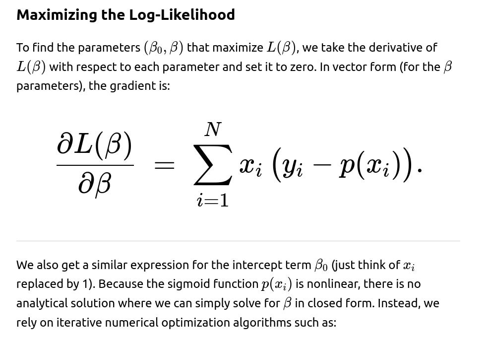
To maximize this, we take derivatives with respect to the parameters and set them to zero. The gradient of the log-likelihood can be written as

Since there is no closed-form solution for β, we solve this numerically using algorithms like gradient descent or Newton-Raphson until convergence.
Comprehensive Explanation
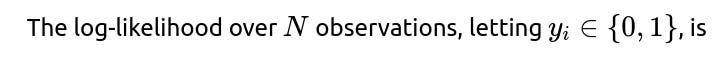
Background of Logistic Regression
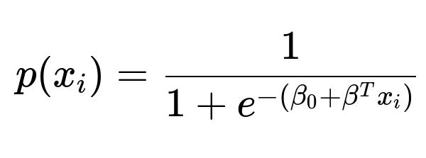
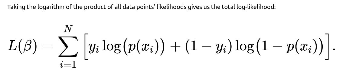
Logistic regression is designed for classification tasks, especially binary classification, by relating the probability of belonging to one class (often denoted class “1”) versus its complement (class “0”). Instead of modeling the output directly with a linear function, logistic regression models the log odds (logit) of belonging to class 1 as a linear function of the features. Specifically, we assume:


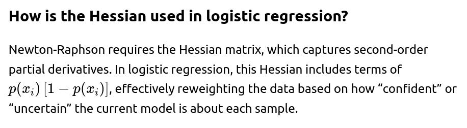
Newton-Raphson (IRLS – Iteratively Reweighted Least Squares)
(Stochastic) Gradient Descent
Quasi-Newton methods (like L-BFGS)
These methods adjust β iteratively in the direction that increases L(β) until convergence.

Potential Follow-up Questions
What distinguishes logistic regression from linear regression for classification?
Linear regression is not well-suited for classification because it can yield outputs outside [0,1] and does not directly model probabilities. Logistic regression ensures outputs are valid probabilities and optimizes the log-likelihood for a Bernoulli-distributed target.

What is the role of regularization in logistic regression?
Regularization (e.g., L2 or L1) adds a penalty term to the loss function that shrinks the parameter estimates. L2 (ridge) regularization penalizes large weights by summing their squares, while L1 (lasso) regularization encourages sparsity by summing their absolute values. This prevents overfitting, improves generalization, and can help in feature selection (L1).
Can logistic regression handle class-imbalanced data effectively?
Logistic regression can be extended to imbalanced data by adjusting class weights or using appropriate sampling techniques (undersampling the majority class, oversampling the minority class, or using Synthetic Minority Oversampling Technique (SMOTE)). One can also evaluate metrics like AUC, precision-recall curves, or F1 score instead of raw accuracy.
Why do we say there is no closed-form solution?
The sigmoid function is nonlinear in the parameters, so the expressions for derivatives do not simplify to a direct solution. Hence, iterative methods are used.
How do we handle multiple classes using logistic regression?
For more than two classes, we generalize logistic regression to multinomial logistic regression (softmax regression). The probability of each class is modeled by exponentiating each linear function and dividing by the sum of exponentials over all classes.
Why is logistic regression’s log-likelihood often called cross-entropy loss in machine learning frameworks?
Maximizing the log-likelihood of the Bernoulli distribution under logistic regression is mathematically identical to minimizing the cross-entropy loss between the predicted probabilities and the true labels.
Are there any convergence issues we might face?
Yes. If features are linearly separable, the log-likelihood can increase indefinitely as certain coefficients grow without bound. In practice, regularization or early stopping (for gradient-based methods) is used to manage this issue.
How do we choose between gradient descent and Newton-Raphson (IRLS)?
Newton-Raphson (IRLS) converges rapidly near the optimum for moderate-sized data, but can be computationally expensive for very large feature spaces or data sets (due to the Hessian).
Gradient Descent variants (batch, mini-batch, stochastic) are more common for very large data sets because they do not require full Hessian computations.
What if the data are not linearly separable?
Logistic regression can still find a decision boundary that best separates the classes in a probabilistic sense. However, if the relationship between features and class label is highly nonlinear, feature engineering or more flexible models (e.g., kernel methods or neural networks) may be required.
How do we handle outliers in logistic regression?
Outliers can significantly affect the estimated coefficients, especially if they strongly influence the log odds. Regularization is often used to combat sensitivity to outliers. Alternatively, robust regression techniques or alternative loss functions could be considered, but classical logistic regression does not inherently ignore outliers.

Why do we say the solution found by logistic regression is a global optimum?
Under typical assumptions (concavity of the negative log-likelihood), there is only one maximum for logistic regression. Thus, gradient-based methods or Newton’s method will converge to the global optimum, not just a local maximum.
Could we use logistic regression as a building block in neural networks?
Yes. The final layer of many neural networks for binary classification is essentially a logistic (sigmoid) layer, turning the network’s outputs into probabilities. Training still involves maximizing a similar likelihood (or minimizing cross-entropy).
How do we handle large-scale data sets with logistic regression?
For very large data, we often rely on stochastic or mini-batch gradient descent. We shuffle the data, process one (or a small batch of) example(s) at a time, and perform more frequent updates to the parameters. This scales better than methods that require full batch computations at each iteration.
Are there any practical concerns about interpretability in logistic regression compared to other models?
Logistic regression is considered more interpretable than many black-box models (e.g., random forests, gradient boosting, deep neural networks). Each coefficient correlates with an odds ratio. However, interpretability may still be limited if the feature set includes complex transformations.
Is logistic regression always the best choice for binary classification?
Not necessarily. If data are extremely high-dimensional, or relationships are highly nonlinear, other methods (like tree-based models or neural networks) might outperform logistic regression. However, logistic regression remains a strong baseline and is often favored for its simplicity and interpretability.
All of these considerations demonstrate how logistic regression’s log-likelihood is derived and optimized, and how we can extend or adapt the method to address real-world complexities.
Below are additional follow-up questions
How does logistic regression handle multicollinearity, and what are potential pitfalls?
Multicollinearity refers to a situation where two or more predictors are highly correlated. In logistic regression, this can lead to unstable estimates for coefficients because the model may struggle to determine which correlated feature is driving changes in the log-odds. Small changes in the data can significantly shift each parameter estimate.
A common symptom of severe multicollinearity is very large absolute coefficient values alongside very large standard errors, indicating instability in those estimates. Despite the overall model possibly still making accurate predictions, interpretation of individual coefficients becomes problematic.
Potential ways to address it:
Regularization (e.g., Ridge/L2): This shrinks the parameters and helps stabilize them when features are correlated.
Dimensionality Reduction: Techniques like Principal Component Analysis reduce the feature space so that it is less prone to collinearity.
Domain-driven Feature Selection: Excluding redundant features based on domain knowledge can help remove correlated predictors.
A pitfall here is dropping potentially important predictors without considering domain knowledge. While dimension reduction might address collinearity, it can obscure interpretability because transformed features no longer correspond to the original predictors.
What if the data has many missing values, and how do we handle them in logistic regression?

Potential handling strategies:
Imputation: Fill in missing values using strategies like mean/median imputation or more sophisticated methods such as k-nearest neighbors or model-based imputation. Pitfalls include bias if the imputation method does not accurately reflect the underlying data distribution.
Indicator Features: Introduce a binary variable to mark whether a certain feature value is missing. Then let the model learn if “missingness” is itself informative. This can help separate missing-at-random from missing-not-at-random scenarios.
Multiple Imputation: Create multiple imputed datasets and average parameter estimates from logistic regression fitted separately on each. This approach can better capture the uncertainty around missing data.
One subtle real-world issue: if data are missing in a systematic way (i.e., not missing at random), naive imputation may lead to biased coefficients. Checking the pattern of missingness is crucial before deciding on the method.
How do we interpret p-values and confidence intervals for logistic regression coefficients, and what edge cases might arise?

Large Coefficients: When data are almost perfectly separable or a feature strongly differentiates the classes, the coefficient can become very large. The standard errors can likewise blow up, making traditional p-values less reliable. Some statistical software will warn of separation or convergence issues in those cases.
Multiple Testing: If testing many coefficients simultaneously (e.g., in very high-dimensional problems), one must adjust for multiple comparisons or risk elevated false positives.
Edge cases arise if the model nearly perfectly classifies the training data with one or more features. In those scenarios, maximum likelihood estimation can push coefficients to extremely large magnitudes, making p-values or CIs questionable. Regularization or removing outliers may help.
How does logistic regression handle very high-dimensional data, and what are best practices for such scenarios?
In high-dimensional settings (where the number of features d can exceed the number of samples N), logistic regression can overfit. Each parameter attempts to adapt to potentially sparse or noisy features.
Best practices:
Regularization: L1 (lasso) helps shrink many coefficients to zero, acting as a form of feature selection. L2 (ridge) shrinks coefficients smoothly while keeping them nonzero. Elastic Net combines both.
Dimensionality Reduction: Techniques like PCA or autoencoders (in deep learning contexts) reduce dimensionality before logistic regression. This helps mitigate overfitting.
Feature Selection: Domain expertise can guide which features matter. Automated feature selection methods, like stepwise approaches, can help but they might be computationally expensive and risk overfitting without careful cross-validation.
A pitfall is that with very high dimensional data, naive unregularized logistic regression might converge to degenerate solutions or never converge reliably. One must carefully tune hyperparameters if using regularization (e.g., the regularization strength) and ensure proper cross-validation for robust performance estimation.
How does logistic regression compare with SVM in terms of performance and interpretability under different data conditions?
Both logistic regression and SVMs can be used for binary classification, but they differ:
Objective: Logistic regression optimizes log-likelihood (equivalently, cross-entropy), yielding probabilistic outputs. SVM tries to maximize the margin (distance between the decision boundary and the support vectors), often focusing on classification accuracy rather than probability estimation.
Interpretability: Logistic regression is typically simpler to interpret because each coefficient has a direct meaning in odds terms. In contrast, the significance of SVM’s support vectors and kernel parameters can be more opaque.
Handling Overlaps/Noise: Logistic regression fits probabilities; when classes heavily overlap, it can still output a well-calibrated probability. SVM with certain kernels can be more flexible in boundary shapes but may require careful hyperparameter tuning.
Scalability: Both can handle large datasets, but SVM might be expensive for very large N, especially with complex kernels. Logistic regression is often easier to scale via stochastic gradient methods.
A subtle edge case arises if you need well-calibrated probabilities rather than just a decision boundary. SVM typically only provides a distance measure, not a direct probability (though one can apply Platt scaling). If interpretability is paramount, logistic regression often wins, but if raw predictive performance in complex feature spaces is the key, certain SVM setups can be more powerful.
How do we check the quality of our logistic regression model beyond standard accuracy measures?
Accuracy can mislead if classes are imbalanced or if certain types of errors are more costly. To get a more complete picture:
Confusion Matrix: Shows true positives, false positives, true negatives, and false negatives. It helps diagnose where the model is making mistakes.
Precision and Recall: Particularly important if one class is rare (e.g., fraud detection). Low recall might mean many missed positive cases, which could be unacceptable in certain applications.
F1 Score: Harmonic mean of precision and recall, balancing both metrics.
ROC and AUC: Plot the true positive rate vs. false positive rate at various thresholds. The area under the ROC curve (AUC) summarizes how well the model ranks positive vs. negative examples.
Calibration: Reliability diagrams and the Brier score check whether predicted probabilities match actual frequencies. Well-calibrated probabilities are crucial in settings like medical diagnoses or financial risk.
A pitfall can be focusing solely on accuracy in highly skewed datasets. For instance, predicting “majority class” for every case might yield high accuracy but is essentially useless for identifying minority cases.
How should we choose the probability threshold for making classification decisions in logistic regression?

Guidelines:
Cost-based: If missing a positive case is more expensive, we might lower the threshold below 0.5, capturing more positives but increasing false positives.
Precision-Recall Tradeoff: One can look at the precision-recall curve to find a threshold that gives an acceptable balance.
Receiver Operating Characteristic (ROC): Varying the threshold sweeps out an ROC curve; the “optimal” threshold might be found by maximizing the Youden index or other metrics.
Business/Domain Considerations: Real-world constraints (e.g., legal, medical, financial) may dictate an acceptable false-positive rate or false-negative rate.
A subtle pitfall is to rely on a universal threshold like 0.5 in a heavily imbalanced scenario. This may yield poor results for the minority class. It is common to choose an operating threshold that reflects domain-specific risk and benefits.
How do we incorporate Bayesian concepts into logistic regression, and what real-world advantages does Bayesian logistic regression offer?
In Bayesian logistic regression, we place priors on the coefficients (e.g., normal priors analogous to L2 regularization, or Laplacian priors analogous to L1). Then we use the observed data to update these priors into posterior distributions over coefficients, often via sampling methods like Markov Chain Monte Carlo (MCMC) or variational inference.
Advantages:
Uncertainty Estimates: Instead of just a point estimate for each coefficient, Bayesian methods provide a posterior distribution, indicating the range of likely values given the data and the prior.
Incorporating Domain Knowledge: One can encode prior beliefs, such as that coefficients should be near zero or within certain ranges, which helps in small-data or noisy contexts.
Regularization via Priors: Priors act as a form of regularization, mitigating overfitting.
However, a pitfall is that Bayesian logistic regression can be computationally expensive, particularly if the dataset is large or the dimensionality is high. Approximate methods like variational Bayes can help but might introduce their own approximation biases.
What strategies exist for diagnosing whether logistic regression has converged properly, and what can lead to non-convergence?
Convergence in logistic regression means that parameter updates are sufficiently small and the log-likelihood stops changing significantly. Common indicators of convergence issues include:
Diverging Coefficients: If parameter magnitudes explode, you may have perfect or near-perfect separation in the data.
Oscillating Loss: The objective function fails to settle, perhaps from an over-aggressive learning rate in gradient descent or numeric instability in Newton-based methods.
Software Warnings: Many libraries (e.g., R’s glm, Python’s statsmodels or scikit-learn) issue warnings about failed or partial convergence.
Possible fixes:
Feature Scaling: Logistic regression optimizers often assume moderately scaled features. Very large or very small feature values can cause numeric issues.
Add Regularization: This can prevent runaway coefficients in cases of near-separation.
Reduce Step Size (Learning Rate): For gradient-based methods, too large a learning rate might cause divergence.
Inspect Data: Look for near-duplicate observations with contradictory labels or extremely high leverage points.
A subtle real-world issue is that if the data truly are separable, the algorithm will push certain coefficients toward infinity, never truly converging. Practical solutions include adding regularization or removing ambiguous or outlying points.
How do we handle categorical variables with many levels in logistic regression, and what pitfalls could arise?
Categorical features need to be encoded before logistic regression can handle them. A common approach is one-hot encoding, where each category becomes a dummy variable. However, if a categorical variable has a large number of levels (high cardinality), one-hot encoding can explode the feature space.
Potential pitfalls:
Overfitting: High-cardinality variables create many parameters that might fit noise, especially with small data. Regularization is often essential to control complexity.
Sparse Data Issues: If certain categories appear rarely, those dummy variables might have insufficient data to estimate meaningful coefficients.
Encoding Schemes: Alternatives like target encoding or frequency-based encoding might be employed. But these can introduce leakage if not done carefully with proper cross-validation.
Edge cases arise when a certain category is extremely rare—there might be nearly complete separation for that category. This can inflate coefficients. Another pitfall is inadvertently introducing perfect collinearity (summing across all dummies yields a vector of all ones), so typically one reference category is omitted.
What is the difference between deviance and residual deviance in logistic regression, and why might these diagnostics matter?
Deviance in generalized linear models, including logistic regression, is defined as twice the difference between the saturated model log-likelihood and the fitted model log-likelihood. The saturated model fits the data perfectly, so deviance measures how far the fitted model is from a perfect fit.
Residual deviance is the deviance remaining after the model is fit; it is effectively the deviance of the fitted model itself. Lower residual deviance indicates a model that is closer to the saturated model. Comparing residual deviance to degrees of freedom sometimes helps detect overfitting or underfitting.
A potential pitfall is over-relying on deviance alone. Large sample sizes can produce statistically significant deviance differences for minor practical improvement. Conversely, small sample sizes may have deviance results that are inconclusive. Always pair deviance-based diagnostics with domain knowledge, cross-validation, or other performance measures.
How might logistic regression be extended to handle ordinal or hierarchical response structures, and what are common pitfalls?
In some tasks, the response variable is not just binary or nominal multi-class, but ordinal (e.g., movie ratings 1,2,3,4,5) or hierarchical. Standard logistic regression does not directly account for the ordering among classes.
For ordinal data, extensions like ordinal logistic regression (e.g., proportional odds model) impose a structure where the log-odds thresholds for each category are ordered. For hierarchical data (e.g., nested groupings), multilevel logistic regression can capture random effects at group levels.
Pitfalls include:
Proportional Odds Violation: Ordinal logistic regression often assumes that effects of predictors are the same across different levels, which might not hold in reality. Violations can lead to biased inference.
Complex Random Effects: In hierarchical logistic regression, specifying random intercepts or slopes can greatly increase model complexity. Convergence issues or identifiability problems may arise if data are limited within some levels.
Interpretation: Coefficients in ordinal or hierarchical models are often more nuanced to interpret compared to standard binary logistic regression. One must carefully articulate the meaning of “thresholds” or “random effects.”
In what scenarios could logistic regression inadvertently produce extremely skewed predicted probabilities, and how can we mitigate this?

Mitigation strategies:
Regularization: Keeps coefficients smaller, reducing the chance of inflated log-odds.
Robust Feature Engineering: Winsorizing or scaling outliers can reduce the effect of extreme values.
Monitoring and Retraining: In production, track input distributions to detect shifts. If necessary, retrain or recalibrate the model on new data.
Platt Scaling or Isotonic Regression: Post-hoc calibration can help “pull in” extreme probability estimates to better match empirical frequencies.
A subtle real-world issue is if you rely on these probabilities for risk predictions (like medical or financial decisions), very large or small probabilities can have drastic consequences. Ensuring well-calibrated outputs is critical.
How can we debug or visualize the decision boundary in logistic regression, and why might such visualization be misleading in higher dimensions?
A typical debug approach is to plot the decision boundary on a 2D scatterplot of features, coloring points by predicted class probability. This can reveal whether the boundary is reasonable.
However, with more than two features, visualizing the decision boundary directly is challenging. One might:
Plot Partial Dependence: Fix some features at typical values and vary one or two features to see how predictions change.
Dimensionality Reduction: Project to 2D with PCA or t-SNE, then overlay logistic regression predictions.
Feature Interaction Analysis: Look at how interactions between pairs of features affect predictions (could be done by grid sampling).
Potential pitfalls:
Loss of Fidelity in High Dimensions: A boundary that seems simplistic in 2D slices may actually be sufficiently complex in full feature space.
Misleading Projections: Dimensionality reduction might distort distances or cluster relationships, leading to an inaccurate depiction of how the boundary truly divides data in the original space.
Such visual checks are still valuable for diagnosing gross model errors (like a boundary that misses an obvious cluster). But in very high-dimensional problems, combining partial dependence plots with domain knowledge may be more practical than purely geometric interpretation.
How can domain-specific knowledge be integrated into logistic regression models?
Domain knowledge can guide:
Feature Selection: Decide which variables are theoretically relevant or define transformations that align with known relationships (e.g., ratio-based features if domain dictates).
Interaction Terms: If we know certain features interact multiplicatively, explicitly include an interaction term.
Custom Encoding: For categorical variables with domain structure (e.g., hierarchical categories), we might group them or use specialized encoding.
Prior Information (Bayesian approach): In Bayesian logistic regression, we can encode beliefs about plausible coefficient magnitudes.
Pitfalls include inadvertently imposing incorrect assumptions or ignoring emergent patterns if domain knowledge is overly restrictive. Additionally, manual feature engineering might be time-consuming or prone to human bias. Cross-validation remains essential to verify that domain-driven modifications genuinely improve predictive performance.
How do we approach logistic regression in a streaming or online learning context?
In streaming or online learning scenarios, data arrive incrementally and the model must update parameters without retraining from scratch:
Online Gradient Descent: Update β after each new observation (or small batch) using the gradient of the log-loss for that observation. This can adapt to changing data distributions in real time.
Adaptive Learning Rates: Methods like AdaGrad, RMSProp, or Adam dynamically adjust the learning rate over time, often helping with convergence.
Warm Starts: Keep the current parameter estimates as the initialization for the next training phase rather than starting from scratch.
Edge cases and pitfalls:
Non-Stationary Streams: If the data distribution drifts, older data might harm performance. Some strategies use forgetting factors or reweighting to emphasize recent data.
Memory Constraints: Storing all past data might be impossible. Properly discarding or summarizing historical data is key to controlling memory usage.
Overfitting Rare Patterns: If a small unusual batch appears, the model might overreact. A stable approach (like slower learning rates or mini-batching) can smooth out extreme fluctuations.