
ML Interview Q Series: Explain the concept of L1 and L2 regularization in machine learning, and discuss how they differ from each other

📚 Browse the full ML Interview series here.
Short Compact solution
In machine learning, both L1 and L2 are approaches to regularization, which helps combat overfitting by shrinking model coefficients. The difference lies in the form of the additional penalty term that is added to the primary loss function. L1 regularization (often called Lasso) uses the absolute values of the weights as a penalty, which can drive some coefficients to exactly zero and thus produce sparsity. L2 regularization (often called Ridge) employs the squared magnitudes of the weights as its penalty, which shrinks coefficients toward zero but usually does not set them exactly to zero. The two loss functions can be written as:
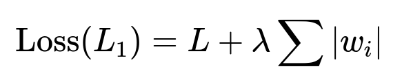

where L is often the sum of squared errors from the prediction task, wi are the model coefficients, and λ is the regularization parameter that balances fitting the data and shrinking the weights.
Comprehensive Explanation
Underlying Idea of Regularization
The main purpose of adding a regularization term to a model’s primary loss function is to reduce overfitting. Overfitting can occur when a model fits not just the true underlying relationship but also the random noise in the dataset. By penalizing large coefficients, we can smooth the solution space and force the model to focus on the most critical relationships.
L1 Regularization (Lasso)
L1 regularization adds a penalty proportional to the absolute values of the coefficients. Because the absolute value function has a cusp (a “sharp corner”) at zero, the gradient-based optimization will often cause some coefficients to become exactly zero if they are not strongly supported by the data. Thus, L1 regularization inherently performs feature selection by zeroing out less important features.
Mathematically, for a given set of weights w=(w1,w2,...,wp) and predictions f(x), the loss with L1 regularization can be:


L2 Regularization (Ridge)
L2 regularization, in contrast, adds a penalty proportional to the squared values of the coefficients. Because squares are smooth around zero, the penalty continuously shrinks coefficients but does not often bring them fully to zero. Instead, it makes large weights smaller and distributes the shrinkage more evenly.
The corresponding loss for L2 regularization can be written as:

The squared penalty grows faster as weight magnitudes increase, leading to a strong incentive to keep weights small overall.
Why L1 Encourages Sparsity and L2 Does Not
A key reason behind L1 regularization’s tendency to produce sparse solutions (exactly zero coefficients) is the shape of its penalty term. The absolute value function has a constant gradient magnitude except at zero itself, where the gradient is undefined but effectively can push the weight directly to zero. In practical gradient-based optimization, once a weight becomes very small, L1 tends to set it to zero to further reduce the penalty cost.
L2 regularization’s penalty is smooth. The gradient of the squared term near zero is also small, so it does not force the coefficient to cross zero in a single large step. Instead, it smoothly pulls all coefficients toward zero without usually causing them to vanish entirely.
Geometric Interpretation

Practical Examples
L1 / Lasso: When the goal is to identify a small set of highly relevant features or when interpretability is important (you want to see a subset of nonzero weights). It excels in high-dimensional settings where you suspect many features are irrelevant.
L2 / Ridge: When you want to reduce model variance and avoid large weights but still keep contributions from all features. Often used when there is no strong reason to believe many features are exactly useless.
Code Illustration
Below is a simple Python example using scikit-learn to show how one might apply L1 (Lasso) and L2 (Ridge) regularization in a linear regression context:
import numpy as np
from sklearn.linear_model import Ridge, Lasso
from sklearn.model_selection import train_test_split

# Generate synthetic data
np.random.seed(42)
X = np.random.randn(100, 5)
true_coeff = np.array([2.0, 0.0, -1.0, 0.0, 3.0])
y = X @ true_coeff + np.random.randn(100) * 0.5

X_train, X_test, y_train, y_test = train_test_split(X, y, test_size=0.2)

# Ridge Regression (L2)
ridge_model = Ridge(alpha=1.0)  # alpha is the regularization parameter
ridge_model.fit(X_train, y_train)
print("Ridge coefficients:", ridge_model.coef_)

# Lasso Regression (L1)
lasso_model = Lasso(alpha=0.1)  # alpha is the regularization parameter
lasso_model.fit(X_train, y_train)
print("Lasso coefficients:", lasso_model.coef_)
In this example, the Lasso model is more likely to show exactly zero coefficients, while the Ridge model simply reduces their magnitude.
What Are Possible Follow-up Questions?
How Does L1 Regularization Aid Feature Selection?
L1 tends to drop many weights to zero, effectively pruning out features. This is particularly useful when the number of features is huge, but we suspect only a few are genuinely relevant. By driving coefficients to zero, L1 automatically performs feature selection within the training process.
If L1 Produces Zero Coefficients, Is It Always Superior for Interpretability?
While L1 can simplify interpretability by producing sparse models, it is not always superior. In certain cases—especially when correlated features exist—L1 may arbitrarily pick one feature over another. If multiple features provide similar information, L1 might zero out some or all of them in ways that can sometimes be unstable without additional considerations, such as group-lasso or elastic net.
When Would We Prefer L2 Regularization Over L1?
L2 regularization is often preferred when:
We do not need a strict sparse solution.
We want to reduce the model variance by distributing shrinkage among all features more smoothly.
We suspect that most features do have at least some relevance, so setting them entirely to zero might be too aggressive.
What Is the Role of the Regularization Parameter λλ?
λ (often referred to as alpha in some libraries) controls the intensity of the penalty. A larger λ means more emphasis is placed on shrinking weights, leading to simpler models (fewer nonzero coefficients in the L1 case, and smaller coefficient magnitudes in the L2 case). A smaller λ allows coefficients more freedom to fit the data closely, potentially risking higher variance and overfitting.
Can We Combine L1 and L2? What Is the Elastic Net?
Yes. Elastic Net is a technique that combines both L1 and L2. Its penalty term is usually a linear combination of the L1 and L2 penalty terms, allowing a model to enjoy both the sparsity of L1 and the smooth shrinkage of L2. It is often applied in situations with many correlated predictors, where pure L1 can behave erratically, and pure L2 may not adequately remove weak features.
How Do We Typically Choose Between L1 and L2 in Deep Learning?
In deep learning, L2 regularization (often called weight decay) is more popular. Neural networks usually have large numbers of parameters, and we often want to reduce the risk of very large weights. Pure L1 can, in principle, help with pruning or compressing models, but it is more commonly used in specialized cases (e.g., to enforce structured sparsity or certain types of feature selection). Another popular alternative in neural networks is dropout, which is a different way to regularize by randomly zeroing out activations during training.
Implementation Challenges and Subtleties
Optimization: With L1, gradient-based optimizers handle the nondifferentiability at zero by using subgradients or specialized optimization algorithms (coordinate descent is commonly used in Lasso).
Scaling of Features: Before applying L1 or L2, standardizing or normalizing features is often crucial to ensure the penalty applies uniformly across all features.
Choosing λ: A cross-validation procedure or a validation set is typically used to select an optimal λ. Finding a balance between bias and variance is a key part of model tuning.
These considerations ensure that L1 and L2 regularization are used effectively in practice.
Below are additional follow-up questions
How do outliers in the dataset affect L1 vs L2 regularization performance?
When there are severe outliers or data following a heavy-tailed distribution, L1 and L2 regularization can behave differently in terms of model stability and coefficient shrinkage. L2 regularization typically penalizes large coefficients more strongly but does not inherently mitigate the influence of outliers on the overall loss function. If an outlier exerts substantial leverage, the model might continue to adjust weights to accommodate it, especially in ordinary least squares with L2. On the other hand, L1 regularization can sometimes help if the solution can “zero out” or drastically shrink the parameter that corresponds to the feature primarily causing the outlier’s influence. However, if an outlier strongly affects multiple features, pure L1 alone might still struggle.
Pitfalls and Edge Cases
Multiple Features Driving Outliers: If an outlier is not tied to just one coefficient, L1 may not be able to isolate and zero out just that single dimension.
Robustness to Large Errors: Neither standard L1 nor L2 is fully robust to extremely large outliers without additional modifications like Huber loss or trimmed means.
Overcorrection: In some cases, L1 might push relevant coefficients to zero if those features appear too volatile due to outliers.
How does feature correlation interplay with L1 vs L2 regularization?
When predictors (features) are highly correlated, L1 (Lasso) may zero out one predictor in favor of another, effectively choosing one correlated feature while discarding others. This can simplify the model but may appear somewhat arbitrary if multiple features are similarly informative. L2 (Ridge) handles correlated features by spreading out the penalty more evenly, shrinking coefficients together rather than setting some of them exactly to zero.
Pitfalls and Edge Cases
Arbitrary Feature Retention: L1 might pick a feature randomly among several correlated features if they are all equally relevant.
Excessive Shrinkage of Important Predictors: With L2, a truly important predictor could be forced to share penalty with correlated variables, potentially underestimating its effect.
Elastic Net: In real-world scenarios with correlation, using a combination of L1 and L2 can mitigate the risk of discarding correlated features while still benefiting from sparsity.
Does L1 or L2 regularization affect bias and variance differently?
Yes, regularization shifts the trade-off between bias and variance. In broad strokes, adding stronger regularization (whether L1 or L2) will generally increase bias but decrease variance. L1 often increases bias more starkly when it completely eliminates certain weights, but this can reduce variance quite effectively. L2 consistently shrinks all coefficients, creating a controlled increase in bias and a usually smoother decrease in variance.
Pitfalls and Edge Cases
Excessively High Regularization: Pushing coefficients to nearly zero or exactly zero can result in underfitting, with high bias and low variance.
Low Regularization: Coefficients might grow unchecked, leading to overfitting and high variance.
Model Complexity: In complex models (e.g., deep neural networks), L2 weight decay can help keep weights smaller, but the potential for high variance might remain if the model architecture is very large.
How do we interpret the final models or coefficients in real scenarios if we used L1 vs L2?
For L1, interpretability often appears more straightforward because some weights are exactly zero, implying those features are excluded from the model. For L2, coefficients tend to be shrunken but not eliminated, providing a more distributed notion of feature importance. However, even in the L1 case, one must be cautious: zeroed coefficients do not necessarily mean the feature has no relationship to the target—it might just be highly correlated with another retained feature or overshadowed by stronger signals.
Pitfalls and Edge Cases
False Sense of Non-Relevance: A coefficient driven to zero by L1 might still be relevant if a correlated feature remains in the model.
Overinterpretation of Small Coefficients: L2 might leave small but non-zero coefficients. Interpreting them as truly meaningful may be questionable if regularization forced their shrinkage.
Domain Knowledge: Practical interpretation should always be combined with domain expertise, especially if features are correlated or if data quality is uncertain.
Is there any difference in the optimization process or required solver for L1 vs L2, particularly in large-scale or online learning contexts?
Yes, L1 regularization involves an absolute value penalty which is not differentiable at zero, so special optimization techniques (e.g., coordinate descent, subgradient methods, proximal gradient methods) are used. L2 regularization, being differentiable everywhere, can be more straightforward to implement with standard gradient-based methods. In very large-scale contexts or online learning, L2 is often simpler to maintain, as its gradients are direct, while L1 might need more nuanced updates to handle the non-differentiable point at zero.
Pitfalls and Edge Cases
Convergence Issues: Poorly chosen learning rates or subgradient approaches can lead to very slow or erratic convergence for L1-based models.
Computational Costs: Coordinate descent is very effective for L1 in moderate dimensions, but extremely high-dimensional data may demand specialized distributed methods.
Online L1: Methods like truncated gradient or proximal operators can be implemented in an online fashion, but they require careful tuning to ensure sparse solutions remain stable.
When dealing with extremely large or extremely small λ values, how might we troubleshoot training and generalization issues for each regularization method?
Extremely Large λ: Both L1 and L2 will heavily penalize coefficients. L1 may quickly drive most of them to zero, causing severe underfitting. L2 will collapse them toward zero, also risking underfitting.
Extremely Small λ: The penalty effect becomes negligible; the model can overfit by growing coefficients large.
Troubleshooting:
Monitor training and validation losses to see if the model is underfitting (suggesting λ is too high) or overfitting (suggesting λ is too low).
Adjust λ systematically, often using cross-validation or Bayesian optimization approaches.
Inspect which features are zeroed out under L1 or which remain large under L2 to understand if the current λ is reasonable.
Pitfalls and Edge Cases
Hardware Constraints: Extremely large λ might push many coefficients to zero in L1, effectively ignoring features that might be critical.
Misinterpretation: Seeing near-zero coefficients in L2 could simply be an artifact of an excessively high λ, rather than a true reflection of feature irrelevance.
Non-Converging Training: In neural networks, a huge L2 penalty (weight decay) might overly constrain learning, leading to potential convergence issues.
Are there certain distribution assumptions behind L1 vs L2 that might reflect typical or special cases in real data?
Though not strict assumptions in a classical statistical sense, there are heuristic interpretations:
L2: Minimizing L2 penalty is akin to a Gaussian prior on the coefficients (in Bayesian terms), assuming weights are likely centered near zero with a normal distribution.
L1: Minimizing L1 penalty aligns with a Laplacian prior, implying many coefficients are exactly or near zero, with a heavy peak at zero in the prior distribution. In some real-world datasets, if you suspect a strong majority of features are irrelevant (leading to truly sparse solutions), a Laplacian prior (L1) might be more suitable. Conversely, if you believe all features should have at least some effect, albeit small, a Gaussian prior (L2) can be more appropriate.
Pitfalls and Edge Cases
Priors Not Representative: Actual data distributions might not match either Gaussian or Laplacian well, making a pure L1 or L2 approach less ideal.
Mixture of Sparse and Dense: In reality, some features are truly zero, and others are distributed around non-zero means. Hybrid approaches like the Elastic Net can better match these scenarios.
How do we select the best regularization technique if we suspect non-linear relationships or if we are using advanced models beyond linear or logistic regression?
For non-linear models (e.g., tree-based methods, neural networks, kernel methods), the concept of L1 vs L2 still applies, but the interpretation is more complex. In tree-based models, L1 or L2 weight penalties may not be as critical, because trees don’t use continuous coefficients. Instead, we might use techniques such as minimal leaf size constraints or max depth constraints. In neural networks, L2 weight decay is common, though L1 can be used to encourage feature-level or neuron-level sparsity.
Pitfalls and Edge Cases
Overreliance on L1/L2 in Non-Linear Contexts: Non-linear models can have many hyperparameters, such as depth for trees or dropout for neural networks, that can overshadow the effect of L1/L2.
Interpretation: Sparsity is less straightforward in deep networks with L1 because setting a single weight to zero doesn’t necessarily “remove” a feature as it does in linear regression.
Hyperparameter Tuning: For advanced models, balancing L1 or L2 with other regularization strategies (dropout, batch normalization, early stopping) becomes a multi-dimensional search problem.