
ML Interview Q Series: Explain the concept of a loss function’s ‘gradient Lipschitz constant.’ Why is this property important for convergence guarantees in gradient-based methods?


📚 Browse the full ML Interview series here.
Hint: Bounded gradients help ensure stable training steps.
Comprehensive Explanation
A function having a gradient Lipschitz constant means that the gradient does not change too abruptly. In a machine learning context, this property helps us ensure that when we make gradient-based updates to parameters, we do not take overly large steps that lead to divergence or instability. Formally, we say a function f(x) (representing our loss) has an L-Lipschitz continuous gradient if the following inequality holds for any pair of points x and y in the domain:

where f is the loss function, x and y are parameter vectors, ∇f(x) is the gradient of f evaluated at x, L is a non-negative real number called the Lipschitz constant, and ‖·‖ denotes an appropriate norm (usually the Euclidean norm in optimization contexts). This means that the difference between the gradients at two different points is bounded by L times the distance between those points.
In gradient-based methods, the significance is that if we choose a step size smaller than 1/L (in basic gradient descent settings), we can guarantee convergence of the parameter sequence to an optimal value (in convex settings) or a stationary point (in non-convex settings). The Lipschitz constant essentially controls how wildly or smoothly the gradient can vary. A smaller L value implies that the gradient changes more gently, allowing larger and more confident steps without overshooting.
When L is very large, the gradient can change drastically with small shifts in the parameter space, requiring more cautious (smaller) step sizes. If the gradient is not Lipschitz continuous (or if L is extremely large), gradient-based methods risk large jumps, oscillation, or divergence.
Practical Considerations
In practice, we often do not know the exact Lipschitz constant for complicated models (like deep neural networks). Still, the concept underpins many optimization and analysis techniques that assume or require bounded gradient changes. Researchers use methods like gradient clipping, adaptive step sizes (Adam, RMSProp), or specialized step-size search algorithms to handle situations where the Lipschitz constant might be large or unknown.
Potential Implementation Example in PyTorch
Below is a short example in Python (PyTorch) demonstrating the idea of gradient clipping. Although not a direct computation of the Lipschitz constant, gradient clipping ensures that gradients remain within a certain norm range. This helps mimic bounded gradient behavior in practice:
import torch

# Suppose we have a model and an optimizer
model = SomeModel()
optimizer = torch.optim.SGD(model.parameters(), lr=0.1)

for batch_data, batch_labels in dataloader:
    optimizer.zero_grad()
    outputs = model(batch_data)
    loss = loss_fn(outputs, batch_labels)
    loss.backward()
    # Gradient clipping to ensure gradients don't explode
    torch.nn.utils.clip_grad_norm_(model.parameters(), max_norm=1.0)
    optimizer.step()
By clipping the gradient to max_norm=1.0, we effectively bound its norm and can maintain a more stable training process akin to having a controlled Lipschitz constant.
Follow-up Questions
How does the Lipschitz condition help in selecting the step size during gradient descent?
A common theoretical result is that if the gradient is L-Lipschitz, a step size that is at most 1/L will ensure stable convergence in convex problems. Intuitively, if you move in the opposite direction of the gradient with a sufficiently small step size, you will not overshoot the minimum. In non-convex settings, choosing a step size inversely related to L can still help you avoid overly large steps and reduce the risk of instability.
Is a Lipschitz continuous gradient enough to ensure global convergence for non-convex problems?
A Lipschitz continuous gradient alone does not guarantee that you will find a global minimum in a non-convex setting. It only provides control over step sizes to prevent divergence and to achieve convergence to a stationary point. Non-convex optimization can have many local minima or saddle points, so additional assumptions (e.g., specific structures in the loss landscape or strong convexity in certain regions) are required for guarantees of global optima.
Does having a gradient Lipschitz constant imply that the function is convex?
A Lipschitz continuous gradient does not necessarily imply convexity. Lipschitz continuity of the gradient is an assumption about how fast the gradient can change, whereas convexity is about the shape of the function with respect to every pair of points in its domain. You can have non-convex functions whose gradients are still Lipschitz continuous. Convexity and Lipschitz continuity of the gradient are separate properties, though they are frequently used together in theoretical analyses of optimization algorithms.
How do we handle situations where we do not know the Lipschitz constant in practice?
Exact computation of L might be impractical for complex models. In real-world scenarios, methods that adaptively control the step size are often used. Algorithms such as Adam, AdaGrad, or RMSProp adjust the effective step size based on gradient statistics, indirectly accommodating scenarios with large or unknown Lipschitz constants. Gradient clipping is another strategy that ensures gradient norm remains within a desirable range, preventing instability.
Does gradient clipping effectively fix the Lipschitz constant in neural network training?
Gradient clipping does not truly alter the underlying Lipschitz constant of the model’s loss function. Instead, it constrains the gradient norm during backpropagation so that updates remain controlled. While this can help address exploding gradients, it is a heuristic that helps maintain stable training rather than a formal guarantee that the function’s gradient is L-Lipschitz over the entire parameter space. It is, however, a practical workaround to keep updates in a safe range.
Below are additional follow-up questions
How does local Lipschitz continuity compare to global Lipschitz continuity, and why might this distinction matter in practice?
Local Lipschitz continuity restricts gradient behavior within a specific region or neighborhood around a point in parameter space. Global Lipschitz continuity applies across all possible parameter values. In practice, for highly complex or very large neural networks, it might be overly restrictive (or practically infeasible) to assume the gradient is bounded uniformly over the entire parameter space. Instead, researchers often rely on local analyses within the region where the parameters are expected to reside during training. This distinction matters because if the model shifts into a region with a significantly higher Lipschitz constant, the learning rate chosen for a smaller local L might suddenly cause unstable updates or divergence.
Potential pitfalls:
• If the training dynamics move parameters far from the initial region, local Lipschitz arguments may no longer hold. • Overly conservative local estimates can slow down learning if the model rarely ventures outside of that region. • Real-world data shifts might push the model into parameter regimes that were not considered in local analysis, requiring re-estimation of gradient bounds.
Can we estimate or approximate the Lipschitz constant for a neural network, and if so, how?
There are heuristic methods and theoretical bounds that aim to approximate the Lipschitz constant for neural networks, such as:
• Spectral norm bounding: A common approach involves bounding the norm of each layer’s weight matrix and using matrix norm properties to get an overall bound. • Layer-wise approximation: For each layer, approximate how much it can expand or compress signals, then combine these per-layer estimates to approximate the overall Lipschitz constant. • Empirical gradient sampling: Randomly sample parameter points in a region of interest, compute gradients, and estimate the maximum rate of gradient change.
However, these bounds are often loose and can significantly overestimate the true constant, leading to overly conservative step sizes. Fine-grained estimates might be computationally expensive, especially for large or deep architectures, so it remains an open challenge to efficiently compute tight and useful Lipschitz bounds in practical settings.
Potential pitfalls:
• Overly large estimates can lead to excessively small learning rates, slowing convergence. • Overly optimistic estimates risk large gradient steps that might cause instability. • The bounds may fail to account for interactions between layers, especially in architectures with skip connections or attention mechanisms.
What is the relationship between smoothness (Lipschitz continuous gradient) and strong convexity, and why might it matter?
Smoothness (having an L-Lipschitz continuous gradient) and strong convexity are two separate but complementary properties that can significantly impact optimization behavior:
• Smoothness: Dictates how gently or abruptly the gradient can change. This ensures that a gradient-based step does not suddenly increase the loss drastically due to an unbounded change in the gradient. • Strong convexity: Implies that the loss has a curvature lower bound, preventing the function from being too flat. This property enforces a unique global minimum (in strictly convex settings) and often improves the rate at which algorithms converge to that minimum.
In a scenario where a function is both L-smooth and m-strongly convex, one can often derive linear convergence rates for gradient descent, meaning the error shrinks at a rate proportional to some constant factor each iteration (under an appropriately chosen step size).
Potential pitfalls:
• Many practical deep learning losses are non-convex, so strong convexity cannot be assumed globally. • Even in convex settings, strong convexity might only hold in a restricted region of parameter space. • Analyzing the intersection of smoothness and strong convexity can become complex when dealing with large-scale or high-dimensional models.
How might noise in stochastic gradient estimates affect the benefits of having a Lipschitz continuous gradient?
When using stochastic gradient descent, each gradient update is an estimate based on a subset of the data (mini-batch) or even a single example. Even if the true gradient of the loss is L-Lipschitz, stochastic noise can cause variance in the updates:
• The Lipschitz condition ensures the true gradient can’t change abruptly with small parameter shifts. However, stochastic noise might still cause large, random deviations in the estimated gradient. • Lipschitz continuity does not guarantee that the variance introduced by random sampling of data is small; it only bounds the difference in true gradients across parameter space.
As a result, even with an L-Lipschitz gradient, one must use techniques like gradually decreasing the learning rate, variance reduction methods (e.g., SGD with momentum, Adam), or large batch sizes to mitigate the variance in stochastic estimates.
Potential pitfalls:
• If the batch size is too small, variance might overshadow the benefits of Lipschitz continuity, leading to erratic parameter updates. • Poorly tuned learning rates can still cause divergence despite Lipschitz continuity if the stochastic noise is large relative to the chosen step size.
How could we exploit information about second-order derivatives (Hessian) in relation to the Lipschitz continuity of the gradient?
If the Hessian (the matrix of second-order partial derivatives) is bounded in norm, this can also imply Lipschitz continuity of the gradient. Specifically, if the Hessian norm is bounded by L in a region, then within that region, the function’s gradient is L-Lipschitz:
• Bounded Hessian norm means that the curvature of the function is bounded, so the gradient does not change faster than a certain rate. • Second-order methods like Newton’s method directly use Hessian information (or its approximation) for more accurate updates, which can sometimes circumvent overly conservative step sizes that are used when only the Lipschitz constant is known. • In practice, exact Hessian calculations might be too costly for large-scale models, but approximate methods (e.g., quasi-Newton) can partially benefit from second-order insights.
Potential pitfalls:
• Large-scale neural networks can have extremely large Hessians, making direct computation infeasible. • Approximations of the Hessian might still be expensive or prone to numerical instability in high dimensions. • Local bounding of the Hessian may fail if the training trajectory moves into a region with significantly higher curvature.
Could a function have a bounded gradient norm but still fail to satisfy the gradient Lipschitz condition?
Yes. A bounded gradient norm means that ‖∇f(x)‖ remains finite for all x in the parameter domain, but this does not necessarily ensure that ∇f(x) does not change abruptly between two different parameter points. For example, there could be situations where the gradient remains within some finite magnitude but oscillates rapidly in direction, violating the Lipschitz condition that controls how the gradient changes between points.
Potential pitfalls:
• Confusing bounded gradients with Lipschitz continuous gradients can lead to erroneous assumptions about convergence guarantees. • Even if the magnitude of gradients is bounded, rapid directional changes might require adaptive or smaller step sizes. • In real-world training, bounding the gradient norm (e.g., gradient clipping) might mask abrupt directional changes that can affect how reliably one can apply theoretical convergence results.
Why might gradient Lipschitz constants vary drastically between different regions of the parameter space in deep networks?
Deep networks, especially those with non-linear activations like ReLU, often create piecewise linear regions in the parameter space. Each region can exhibit a different local slope behavior, leading to stark variations in how quickly gradients change. Additionally, skip connections, batch normalization, or attention mechanisms can result in complex interactions that affect the local curvature and effectively alter the Lipschitz constant from one region to another.
Potential pitfalls:
• A single global Lipschitz constant might be so large as to be useless in practice, because it reflects worst-case behavior. • Large differences in local curvature can cause training instabilities if the step size is tuned for one region but inadvertently enters another region with a larger Lipschitz constant. • Mechanisms like batch normalization can shift these regions dynamically as the batch statistics evolve, complicating attempts to maintain stable step sizes.
Could adaptive gradient methods like Adam or RMSProp automatically deal with large Lipschitz constants?
Adaptive methods adjust the effective step size per parameter dimension by accumulating statistics of the gradient’s magnitude over time. While this can help manage exploding or large-magnitude gradients, it does not explicitly control how quickly the gradient changes between parameter points. Adam or RMSProp can still face instability if the function’s gradient changes extremely abruptly. They are robust in many practical settings, but they do not provide the same theoretical guarantee as having an actual bound on the gradient’s rate of change.
Potential pitfalls:
• Extremely sharp minima or saddle regions can still cause numerical issues even with adaptive methods. • The hyperparameters (like beta1, beta2 in Adam) may need careful tuning when gradients exhibit strong fluctuations. • Adaptive methods might mask the need for better architecture design or more direct control of gradient behavior, leading to reliance on heuristics instead of theoretical guarantees.
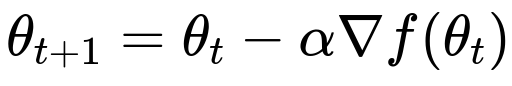
Above is the standard gradient descent update rule in big h1 font. The parameter vector at time t+1 is given by theta_{t} minus alpha times the gradient of f evaluated at theta_{t}. In practice, to ensure this update does not produce divergence, alpha typically must be chosen to be smaller than or equal to 1/L if the gradient is L-Lipschitz and the problem is convex. If the Lipschitz constant is not well known or is very large, choosing alpha can be challenging, and techniques like adaptive optimization or gradient clipping become attractive alternatives.