
ML Interview Q Series: Explain the core concept of PCA, its matrix formulation and derivation, iterative procedure, and constrained optimization.

📚 Browse the full ML Interview series here.
Short Compact solution

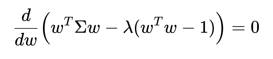
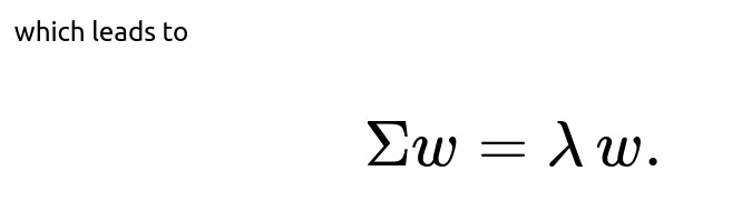
Thus ww must be an eigenvector of Σ, with the eigenvalue λ indicating the variance along that direction. The principal components are determined by selecting the eigenvectors corresponding to the largest eigenvalues, ensuring that each subsequent component is orthogonal to the previous ones. In practice, the first few principal components capture most of the variance, allowing us to reduce the data to k dimensions.
Comprehensive Explanation
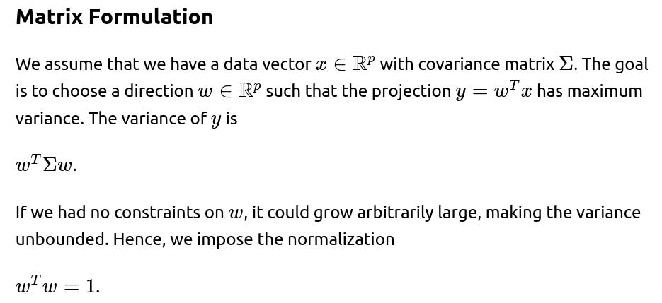
Principal Component Analysis (PCA) is a technique used to simplify data by mapping it into a lower-dimensional subspace that retains most of the meaningful structure (variance) of the original data. The key is to identify new, orthogonal directions that capture maximal variance, and then project the data onto these directions.
Reasoning Behind PCA
In high-dimensional datasets, there can be redundancy, where many of the original features are correlated or do not add much information. PCA addresses this by finding new axes (directions in feature space) that contain as much of the original data’s variation as possible. By restricting attention to the top k such axes, one reduces dimensionality while still preserving most of the variability in the data.

Iterative Procedure
To find multiple principal components, we pick the first component by taking the eigenvector corresponding to the largest eigenvalue of Σ. We then find the second principal component by taking the eigenvector corresponding to the second largest eigenvalue, and so on. By construction, these eigenvectors are all orthogonal (or can be chosen to be so if there are ties). This procedure yields a basis of principal components.
Practical Significance
In real-world settings, data often has dimensions in the hundreds or thousands, and many of these dimensions are correlated or only add marginal information. PCA allows us to reduce the dimensionality, often to a much smaller number of components, while retaining most of the variation of the original dataset. This can significantly improve computational efficiency, remove noise, and reveal underlying structure in the data.
Example Implementation in Python
import numpy as np

def pca(X, k):
    # Assume X is an n x p data matrix, with rows as data samples
    # Center the data by subtracting the mean
    X_centered = X - np.mean(X, axis=0)

    # Compute covariance matrix
    Sigma = np.cov(X_centered, rowvar=False)

    # Eigen-decomposition
    eigenvalues, eigenvectors = np.linalg.eig(Sigma)

    # Sort eigenvalues (and corresponding eigenvectors) in descending order
    idx = np.argsort(eigenvalues)[::-1]
    eigenvalues = eigenvalues[idx]
    eigenvectors = eigenvectors[:, idx]

    # Select the top k eigenvectors
    W = eigenvectors[:, :k]

    # Transform the data into the new subspace
    X_pca = np.dot(X_centered, W)
    return X_pca, W, eigenvalues[:k]
This function returns the dimensionality-reduced data X_pca, the principal component directions W, and the top k eigenvalues. Typically, one then examines the fraction of total variance explained by these eigenvalues to decide how many components k are sufficient.
Why the PCA Directions are Orthonormal
Each principal component is an eigenvector of the covariance matrix Σ. By definition, distinct eigenvectors of a symmetric matrix (like Σ) corresponding to distinct eigenvalues are orthogonal. Additionally, each eigenvector is normalized to have unit length. Therefore, these directions automatically form an orthonormal set.
Follow-up question: How does centering (subtracting the mean) affect PCA?
Centering the data is crucial because PCA depends on the data’s variance being correctly represented by the covariance matrix. If the data is not centered, the covariance matrix may not capture relationships accurately, and the principal components might not align with the directions of maximal variance in the intended manner. By subtracting the mean, we ensure that the covariance matrix is a true reflection of variances and covariances around the origin. This leads to principal components that correctly represent the directions of maximal variation.
Follow-up question: Why do we typically use the covariance matrix rather than the raw data for PCA?
The main reason is that PCA seeks directions that account for variations in the data. The covariance matrix Σ concisely encodes how each dimension in the data co-varies with every other dimension. Eigenvectors of Σ thus directly correspond to directions where variance is maximized. Directly operating on the raw data matrix can be more computationally expensive, especially if the dataset is large, although in practice people often rely on the Singular Value Decomposition (SVD) of the data matrix, which is closely related to the covariance-based approach.
Follow-up question: Can we perform PCA without explicitly forming the covariance matrix?
Follow-up question: How can we choose the number of principal components k?

Follow-up question: What are some limitations or pitfalls of PCA?
PCA is a linear method, so it may not capture complex, nonlinear relationships. If data is not scaled properly, or if features have vastly different ranges, the directions found may be skewed. Also, the directions of maximum variance do not necessarily align with directions that best separate classes (if you are doing a classification task). PCA is unsupervised, so it does not incorporate label information. In addition, if the largest variance in the dataset is due to noise, PCA might allocate principal components toward capturing that noise. It’s also important to ensure your data is centered (and possibly standardized) before applying PCA.
Follow-up question: Why can the largest eigenvalue sometimes capture mostly noise?
In some datasets, especially those with a strong source of random variation or an outlier phenomenon, the direction of greatest variance may well be dominated by noise rather than meaningful signal. This occurs if the magnitude of that noisy dimension dwarfs other natural variations in the data. One might mitigate this by standardizing features, removing outliers, or using more robust dimensionality reduction methods such as Robust PCA or methods that incorporate domain knowledge.
Follow-up question: How would you apply PCA in high-dimensional scenarios where p is very large compared to n?
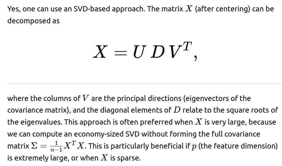
In cases where p≫n, forming the full p×p covariance matrix can be expensive. Instead, one typically uses either randomized PCA or the SVD-based approach on the n×p matrix directly. Randomized PCA uses stochastic techniques to approximate the principal components efficiently and avoid large memory or computational overhead. SVD-based approaches can leverage the fact that the rank of the data matrix may be at most min(n,p), so one can compute the needed truncated decomposition much more quickly.
Follow-up question: How can PCA be used in conjunction with neural networks or deep learning?
One common approach is to perform PCA for dimensionality reduction prior to feeding data into a neural network, particularly when the number of input features is huge. This can help the network train faster by reducing the dimensionality and noise in the data. Another scenario is to analyze latent representations (for example, in autoencoders or large language models) by applying PCA to the hidden representations or embeddings to visualize or interpret them. PCA can also aid in diagnosing issues like covariance shifts or degenerate directions in layer activations.
Follow-up question: What if the data is not well-approximated by a linear subspace?
If the underlying data distribution is highly nonlinear, PCA may not capture the main structure effectively because it only projects onto a linear manifold. In such cases, kernel PCA or other manifold-learning techniques (such as t-SNE, UMAP, or autoencoder-based methods) may better preserve the relevant variations. These approaches use nonlinear transformations or similarity-based techniques to find structure that is not explainable by purely linear directions.
Follow-up question: When implementing PCA, is it always necessary to rotate or whiten the data?
Whitening is sometimes done after PCA by scaling each principal component to have unit variance. This can be useful in certain algorithms, especially in neural network initializations (e.g., in some forms of independent component analysis). However, whitening can introduce noise amplification if small eigenvalues are scaled up too heavily. Rotation (where you simply post-multiply by an orthonormal matrix) does not alter the information content; it’s sometimes used for interpretability, but is not always essential. The main goal of PCA is often just to reduce dimensionality and keep the directions in which the data has the most variance.
Below are additional follow-up questions
How does PCA handle missing data in the dataset?
Handling missing data is not inherently part of PCA’s formulation, since PCA requires complete rows (or an imputation strategy) to compute the covariance matrix or perform SVD. If some data entries are missing, there are various approaches:
Complete-case analysis (listwise deletion): Remove rows that have missing values. However, this reduces the amount of data, potentially biasing the analysis if the data are not missing completely at random.
Imputation methods: Use statistical approaches (e.g., mean, median, KNN-imputation, or more advanced multiple imputation techniques) to fill in missing values. After imputation, you can run PCA on the completed dataset. This relies heavily on how accurately you can estimate the missing entries.
Expectation-Maximization (EM) PCA: A specialized approach that iteratively estimates the missing values while computing principal components. The EM algorithm alternates between estimating missing entries based on current PCA factors, then updating the PCA factors based on these estimates. This can be more efficient and can yield better estimates than simple imputation, but is more complex to implement.
Robust PCA or matrix completion methods: For certain cases (e.g., large structured matrices), you can use matrix completion algorithms that are designed to handle missing entries, producing a low-rank approximation akin to PCA.
A potential pitfall is that each imputation method (or deletion method) can introduce bias or reduce variance. If a large portion of data is missing, you might lose the representativeness of your dataset or incorrectly infer principal directions if the missingness is systematic.
What if your data includes ordinal or categorical variables? Is PCA still appropriate?
PCA is fundamentally a linear method that relies on computing variances and covariances of numerical features. For categorical or ordinal features:
Ordinal variables: Treating them as continuous might distort relationships, especially if the numeric labels do not strictly reflect equal spacing between categories. You can sometimes apply PCA after encoding the ordinal feature as integers, but this can be misleading if the numeric scale doesn’t match the actual underlying relationships.
Nominal categorical variables: Simply encoding them into one-hot vectors and applying PCA can be tricky. The variance-based approach may not be meaningful for variables that lack an inherent numeric scale. Also, if you have many categories, you might inflate dimensionality.
Alternatives might include Multiple Correspondence Analysis (MCA) or Factor Analysis of Mixed Data (FAMD) that handle categorical data more explicitly. A potential pitfall in forcing PCA on purely categorical data is that you may derive spurious directions that do not map well to interpretable, meaningful variation in the data.
Why might some principal components have negative loadings, and does that imply an error?
Negative loadings are completely normal in PCA. Loadings reflect how strongly (and in which direction) each original feature contributes to a principal component. A negative loading simply means that an increase in that feature correlates with a decrease in the principal component score (assuming other features are held constant). It does not imply anything is wrong mathematically or numerically.
An edge case could occur if you see extreme loadings (very large positive or negative values) that might suggest outliers or a near-singular covariance matrix. This is worth checking, but negative loadings by themselves are not a sign of error.
How do we store a trained PCA model and apply it to new data in a production environment?
When you train PCA on a dataset, you typically obtain:
The mean vector (of shape p, where p is the original dimensionality).
The principal components (eigenvectors) (a p×k matrix if you keep the top k components).
Possibly, the eigenvalues (which can be used to track explained variance).
To apply PCA to new incoming data, you first subtract the stored mean from each new sample, then multiply by the matrix of principal components. In code:
# Suppose we have new data point new_x (shape p)
# pca_mean, pca_components from the trained PCA
centered_x = new_x - pca_mean
reduced_x = np.dot(centered_x, pca_components)
A pitfall is forgetting to apply the exact same centering (and optional scaling) that was used during training. Failing to maintain consistent preprocessing pipelines can lead to incorrect projections and inconsistent results between training and inference.
How does PCA deal with outliers, and what issues can arise?
PCA is sensitive to outliers because it relies on the covariance matrix, which is in turn vulnerable to extreme values. An outlier can produce a large shift in the principal directions if it exerts a high leverage effect on the covariance structure.
Potential pitfalls include:
Dominance of outliers: A single or few outliers might pull the principal components toward themselves, overshadowing the broader structure of the majority of the data.
Misleading variance estimates: Variance may become inflated by extreme data points, causing PCA to identify directions dominated by outliers rather than meaningful variation.
Robust PCA variants or data cleaning (e.g., removing or downweighting outliers) can help address these issues. Always examine whether outliers are genuine (meaningful) or measurement errors before deciding on a course of action.
Does PCA produce unique solutions when some eigenvalues are equal?
If there are repeated eigenvalues, the corresponding eigenvectors can be combined in many ways to form valid principal directions. Specifically, any orthonormal basis that spans the eigenspace associated with a repeated eigenvalue is a valid set of solutions.
While numerically you’ll get some specific vectors from an eigen-decomposition algorithm, mathematically the solution in that eigenspace is not unique. In practice, this does not usually cause problems for dimensionality reduction—any orthogonal basis spanning that eigenspace preserves the variance. However, for interpretability or consistency across runs, the non-uniqueness might cause slight confusion if the decomposition changes sign or orientation from one run to another.
How do we interpret principal component loadings in a complex dataset?
After computing PCA, each principal component can be viewed as a linear combination of the original features. The loading vector indicates how strongly each feature influences that principal component. Large (positive or negative) loadings signal that those features have a strong influence on that axis of variation.
Pitfalls include:
Over-interpretation: A large loading doesn’t always imply a causal relationship—correlations among features can also produce large loadings.
Sign or direction: Negative loadings might just mean an inverse correlation with that principal component.
Complex combinations: If you have many features, each principal component might be a combination that is not easily interpretable without domain expertise.
Nevertheless, loadings can provide insights into which features drive major variations in the data, guiding feature selection or domain interpretation.
Is PCA impacted by whether features have highly different units or scales?
Yes. PCA maximizes variance in the original measurement scale of each feature. If some features have large numerical ranges while others are tiny, the large-range features might dominate the first few principal components simply because they contribute more to overall variance. Consequently, standardizing each feature to have mean 0 and unit variance (z-score scaling) before applying PCA is often recommended.
Pitfalls:
Failure to scale: This can overshadow relevant directions in low-scale features.
Over-scaling: In some cases, it might be essential to preserve the actual scale of the data (e.g., if certain features are intrinsically more important). Blindly standardizing might lose that information.
In which scenarios might you prefer Factor Analysis over PCA?
Factor Analysis (FA) and PCA share similarities, but differ in their underlying assumptions and goals. PCA is purely about describing maximal variance in the observed variables via linear combinations. Factor Analysis assumes that observed variables are driven by a smaller set of latent factors plus some noise. FA models the covariance structure with explicit noise terms on each observed variable.
You might prefer Factor Analysis when:
You have a theoretical basis suggesting that a small number of latent constructs underlie the observed variables.
You want explicit modeling of measurement error or unique variances for each observed variable.
Pitfalls:
Incorrect model: If the data is not well-modeled by the Factor Analysis framework, forcing it might produce misleading factors.
Convergence and identifiability: Factor Analysis can have rotation ambiguities and local minima, depending on how it’s implemented.
If the data distribution is non-Gaussian, does that invalidate PCA?
PCA does not strictly require normality assumptions to find directions of maximal variance. The computation of the covariance matrix and its eigenvectors is valid for any real-valued data distribution. However, if the data distribution is heavily skewed, multimodal, or contains strong nonlinear structure, PCA might not capture the “true” patterns effectively.
Pitfalls:
Interpretation: If you assume normal distributions to interpret principal components (e.g., confidence intervals or certain probabilistic inferences), non-Gaussian data can invalidate those interpretations.
Nonlinear complexity: Strongly nonlinear data might require kernel PCA or other manifold learning methods to expose underlying patterns.
How do we handle a situation where we want to visualize data in two dimensions but the first two principal components do not give a good separation?
When using PCA for visualization, it is common to plot the first two principal components. However, these might not always provide meaningful separation or cluster structure, especially if the most significant variances do not align with easily separable clusters.
Potential strategies:
Check higher PCs: Perhaps the first and second PCs are overshadowed by a single dominating direction of variance. Sometimes the third or fourth PC might separate clusters better.
Use domain-specific transformations: Instead of raw data, you might consider derived features or apply transformations before PCA.
Try nonlinear methods: If the separation is inherently nonlinear, consider t-SNE, UMAP, or kernel PCA for potentially clearer cluster separation.
A subtle issue is that PCA is a global linear method, so if the interesting cluster structure is hidden in lower-variance directions, the standard 2D PCA scatter plot might be misleading.
How do we detect how many components we actually need if there is no clear “elbow” in the scree plot?
Choosing the number of components can be challenging, especially if the scree plot (which plots eigenvalues in descending order) doesn’t exhibit a sharp elbow. Some approaches include:
Threshold on explained variance: Select enough components to explain, say, 95% of the variance. But this can be arbitrary and might include noise dimensions if the tail of the spectrum is long.
Cross-validation: Treat the PCA reconstruction error as a metric and use cross-validation to determine how many components minimize the reconstruction error without overfitting noise.
Parallel analysis: Compare the eigenvalues with those obtained from randomly generated data of the same shape. Retain only components whose eigenvalues are larger than the random data’s average eigenvalues.
Domain knowledge: Often, the best approach is guided by practical constraints and interpretability needs.
A pitfall is that purely data-driven criteria can lead you to retain too many or too few components. Balancing interpretability, performance, and domain context is crucial.
Are there situations where PCA might not reduce computational cost significantly?
Yes. Although PCA reduces the dimensionality of the data, the computational cost of finding the principal components can be high if p or the number of data points n is very large. While a smaller dimensional space speeds up subsequent tasks, the initial decomposition step can be expensive:

Sparse or streaming data: Standard PCA can be inefficient if data is continuously streaming or only partially available in memory. Incremental PCA or randomized PCA can mitigate these issues.

A pitfall is to assume PCA always speeds up the workflow. The dimensionality reduction is beneficial after the initial decomposition, but the up-front computation might be prohibitive for extremely large-scale problems unless specialized methods (randomized or incremental PCA) are employed.
What is the relationship between PCA and low-rank matrix approximations?

The pitfall is that if one does not carefully manage the centering or if one confuses row-based or column-based interpretations, one might incorrectly interpret U, D, and V in the context of principal components. Always confirm whether you are doing row-wise vs. column-wise data orientation in the matrix.
Under what circumstances might PCA be detrimental to downstream tasks, such as regression?
PCA is unsupervised, so it identifies directions of maximal variance without considering the relationship to the target variable in a supervised learning task. Potential pitfalls include:
Loss of predictive features: Some features with small variance might actually be crucial for predicting a certain label. PCA might discard or downweight them.
Over-simplification: If you reduce to very few PCs, you might oversimplify the structure that the downstream model requires.
Misalignment: The principal components that maximize overall variance might not align well with the directions that separate classes or predict the target in regression.
In supervised tasks, Partial Least Squares (PLS) or Supervised PCA might be more suitable alternatives if the goal is to retain the directions most relevant to the output variable.