
ML Interview Q Series: Explain the concept of entropy and information gain in decision trees, and illustrate them with a concrete numeric example
📚 Browse the full ML Interview series here.
Short Compact solution
Entropy is a measure of how disordered or mixed a sample is, typically applied to the distribution of class labels. For a simple binary classification with labels a and b, the formula computes how evenly the labels are distributed. A completely homogeneous set (all a’s or all b’s) has entropy 0, while a perfectly balanced 50–50 set has entropy 1.
Information gain (IG) is the drop in entropy that occurs when splitting the data on a particular attribute. You calculate the overall entropy before the split and subtract the weighted sum of entropies of each sub-part after the split.
For example, suppose you have 5 instances of label a and 5 instances of label b (so the total entropy is 1 for a 50–50 distribution). If you split on an attribute X that partitions the data into two groups—one with 5 a’s and 1 b, and another with 0 a’s and 4 b’s—then you compute the entropy of each group and weight them by the fraction of the total. The first group’s entropy is about 0.65, while the second group’s entropy is 0 (since it’s all b’s). After weighting these entropies by 6/10 and 4/10, the overall entropy after splitting is about 0.39. Therefore, the information gain is 1 − 0.39 = 0.61.
Comprehensive Explanation
Entropy in a decision tree measures the degree of impurity in a subset of training examples. When we talk about a binary classification problem with two classes, a and b, the entropy can be expressed (in base 2) as:
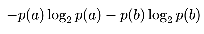
where ( p(a) ) is the proportion of examples labeled a in that subset, and ( p(b) ) is the proportion labeled b. If there are multiple classes, the same concept extends to more terms in the summation.
A crucial idea is that entropy equals 0 when all examples in the subset share the same class, indicating zero disorder or uncertainty about the label. The maximum value of entropy, for a binary setting, is 1, which happens when the number of a’s and b’s in that subset are evenly split.
Information gain measures the change in entropy when we split the data according to a particular feature or attribute. It is computed as:

Here, ( \text{Entropy}(Y) ) is the entropy of the dataset before splitting, and ( \text{Entropy}(Y \mid X) ) is the weighted sum of entropies of each branch after partitioning the data based on feature ( X ).
To illustrate: There are 10 total instances, 5 labeled a and 5 labeled b, so the entropy before any split is 1 (a perfectly even distribution). Suppose the dataset is divided by an attribute X into two subsets: • Subset 1 (X = 1): 5 a’s and 1 b • Subset 2 (X = 0): 0 a’s and 4 b’s
Subset 1 has 6 instances with a proportion of 5/6 for class a and 1/6 for class b. Plugging in those values gives an entropy of about 0.65. Subset 2 has 4 instances, all labeled b, so its entropy is 0. Weighting by each subset’s fraction of the total (6/10 and 4/10) and summing yields an overall post-split entropy of around 0.39. Consequently, the information gain from splitting on this attribute is 1 − 0.39 = 0.61.
In practical terms, a decision tree algorithm evaluates various candidate attributes to split the data and chooses the attribute whose split yields the greatest decrease in entropy (i.e., the highest information gain). A feature that perfectly segregates the labels into pure groups (entropy 0) yields a maximal gain.
Potential Follow-Up Questions
What are possible issues when using entropy and information gain with many-valued attributes?
A concern arises if an attribute takes on many distinct values (for example, an ID field or a timestamp). Such attributes may lead to splits that create very small partitions, each being homogeneous. While this might artificially inflate information gain (because each small partition can have low or zero entropy), it generally does not generalize well. One standard approach to mitigate this is to use information gain ratio, which normalizes the information gain by the intrinsic information of the split, preventing attributes with many distinct values from appearing too powerful.
How do we extend entropy and information gain to more than two classes?
The idea is the same. For a dataset with more than two classes, you sum up the probabilities of each class multiplied by the negative log of that probability. In other words, replace the a/b terms by a summation over all classes. The maximum entropy occurs when all classes have exactly the same proportion of examples, and the minimum entropy (0) occurs when all examples belong to a single class.
Why do we often use log base 2 in the entropy formula?
Log base 2 is typically used because it measures disorder in bits, which is a convenient interpretation from an information theory perspective. In practice, any log base can be used, but base 2 is the standard convention in information theory. If a different base were used, it would just scale the entropy values by a constant factor, which would not affect the relative comparisons for choosing a feature.
Can we quickly demonstrate this calculation in Python code?
Below is a short Python script to compute entropy and information gain for the given example:
import math

def entropy(probs):
    return -sum([p * math.log2(p) for p in probs if p > 0])

def information_gain(total_distribution, subsets):
    # total_distribution: a list of counts for each class in the entire dataset
    # subsets: a list of lists, each sub-list is the counts for each class in a subset

    total_count = sum(total_distribution)
    total_entropy = entropy([count/total_count for count in total_distribution])

    weighted_entropy_sum = 0
    for subset in subsets:
        subset_count = sum(subset)
        subset_probs = [count/subset_count for count in subset]
        weighted_entropy_sum += (subset_count / total_count) * entropy(subset_probs)

    return total_entropy - weighted_entropy_sum

# Example: 2 classes, labeled 'a' and 'b'.
# overall: 5 a's, 5 b's
# subsets: X=1 => 5 a's, 1 b; X=0 => 0 a's, 4 b's

overall_counts = [5, 5]
subset1_counts = [5, 1]  # X=1
subset2_counts = [0, 4]  # X=0

ig = information_gain(overall_counts, [subset1_counts, subset2_counts])
print("Information Gain:", ig)
When you run this code, you get approximately 0.61 as the information gain, matching the manual calculation. This demonstrates how you might programmatically compute entropy and IG.
What is the relationship between Entropy, Cross-Entropy, and KL-Divergence?
In machine learning, cross-entropy measures how one probability distribution diverges from a second, reference distribution. When the reference distribution is the empirical distribution (the observed labels in the dataset), cross-entropy reduces to entropy plus an extra term that measures the mismatch. KL-Divergence (Kullback–Leibler Divergence) is closely related: it is the difference between cross-entropy and the true entropy. In decision trees, we typically deal only with the empirical distribution of classes and measure its disorder with entropy, but in broader deep learning contexts (e.g., classification with neural networks), cross-entropy and KL-Divergence become more relevant.
Are there any practical concerns when computing log probabilities for very small p?
For extremely small probability values, floating-point underflow can occur. While this is typically not a big problem for small-to-medium datasets in decision trees, it can appear in certain large-scale or high-precision contexts. Methods like adding a small epsilon to probabilities or using log-sum-exp tricks (common in deep learning frameworks) are standard ways to handle numerical stability issues.
How can missing data or continuous features be handled when computing entropy-based splits?
Decision trees can handle missing data in various ways. One approach is to split the data into known and unknown partitions. Another is to use statistical imputation or distribute the instance proportionally across children during training. For continuous (numeric) features, algorithms typically evaluate candidate splits by sorting the values and trying threshold-based splits, each time computing the resultant subsets and their entropies. The attribute selection then proceeds just as with nominal features, using the best threshold that leads to the highest information gain.
Below are additional follow-up questions
How does the computational complexity of calculating entropy and information gain scale with dataset size and feature dimensionality?
When computing the entropy for each feature’s potential splits, a decision tree algorithm typically needs to:
Count the distribution of class labels within each candidate split (i.e., how many instances of class a, class b, etc. go left or right, or into each discrete bin).
Compute the probabilities of each class in each split segment.
Use those probabilities to calculate entropy for each segment and then form a weighted sum.
For continuous features, algorithms often consider multiple thresholds, sorting the feature values first and then scanning through potential breakpoints. Sorting requires (O(N \log N)) time for each feature with (N) data points, and checking each potential split in a single pass is (O(N)), so the complexity can be (O(F \cdot N \log N)) for (F) features in a simple implementation. For discrete features with many categories, each category might be its own potential branch, or we might try grouping categories, which can also be expensive.
Potential Pitfalls and Edge Cases
Large Datasets: As (N) grows into millions or billions of records, a naive approach becomes infeasible. Memory constraints come into play if all calculations are kept in memory.
High-Dimensional Data: If (F) is very large (thousands or more features), iterating over each feature for every node can be extremely slow.
Sparse Features: In real-world tasks like text classification (e.g., bag-of-words), many features are 0 most of the time. Efficient data structures or sampling-based approximations may be needed for speed.
Sampling Approaches: Some production-level implementations sample the dataset or features to build approximate trees more quickly (e.g., extremely randomized trees or approximate distribution counting).
How can incremental or streaming data be handled when updating entropy and information gain?
When data arrives in a streaming fashion or changes over time, we may want to update a decision tree’s splits without fully rebuilding the tree from scratch. In principle, one could maintain sufficient statistics (counts of how many examples fall into each branch and class combination) and update them as new data arrives. Then:
Recompute the probabilities of each class in each leaf.
Recompute or approximate the change in entropy and decide if a split is still the best or if a new split is better.
Potential Pitfalls and Edge Cases
Data Distribution Shift: If the underlying distribution changes over time (concept drift), the previously chosen splits may become suboptimal. A naive incremental update might not detect this if it only accumulates counts.
Delayed Labeling: In some streaming contexts, class labels arrive with a delay. Updating entropy on partially labeled data can be challenging—there’s a risk of building splits based on incomplete information.
Computational Overhead: Recomputing information gain for all candidate splits at every new data point is costly. Typically, algorithms use heuristic or time-based triggers to decide when to re-check splits.
Memory Budget: Keeping counts for each node in the tree for large, continuously arriving data can grow big quickly, so an online or approximate approach might be needed.
In what ways might class imbalance influence entropy-based splitting, and how can we address it?
Class imbalance means one class (or a few classes) makes up most of the data, while other classes are rare. Entropy will reflect this imbalance. If 95% of instances are of class a and only 5% are of class b, the initial entropy might still be quite low because one class already dominates. In such a scenario, an attribute split that isolates b doesn’t always look beneficial in a simple entropy comparison because the subset containing b might be small, meaning its weight in the average is small.
Potential Pitfalls and Edge Cases
Minority Class Overlooked: The tree might focus on splitting among the majority class, leaving the minority class with insufficient discrimination.
Overfitting to the Majority: The minority class might get lumped together in a single branch. This can happen if the algorithm aims primarily to reduce overall entropy, ignoring misclassification of the minority.
Metrics: For highly skewed data, accuracy or straightforward information gain is not always the best guide. Balanced metrics like weighted entropy or using cost-sensitive splitting can be more appropriate.
Possible Solutions
Cost-Sensitive Learning: Impose a higher penalty for misclassifying the minority class, effectively “rebalancing” the entropy computation.
Stratified Sampling: If practical, collect a balanced or near-balanced training set.
SMOTE or Oversampling: In some tasks, synthetic data generation or oversampling the minority can help.
Alternative Criteria: Other measures, such as the Gini impurity or even specialized metrics, might handle imbalance differently but still can suffer from the same fundamental issue.
What if we need to incorporate different misclassification costs for various classes during tree construction?
In many real-world scenarios (like medical diagnosis, credit card fraud detection, etc.), different classification errors come with different monetary or societal costs. Traditional entropy-based splitting treats all classification errors equally. To account for different costs:
Weighted Entropy: Assign a cost or weight per class. So, the probability distribution in the entropy formula is weighted by the class’s cost.
Post-Processing: Build the tree using standard entropy, then adjust predictions in the leaves using cost-based thresholds. This is simpler but may not produce the optimal tree structure.
Potential Pitfalls and Edge Cases
Tuning Cost Weights: Determining the right cost ratio can be tricky in practice and may require domain expertise or guesswork.
Rare but High-Cost Classes: If a class is extremely rare but has huge misclassification cost, the model might heavily focus on this class, potentially hurting overall performance on other classes.
Dynamic Costs: Costs sometimes change over time. The tree might need recalculations or partial retraining to reflect new cost structures.
Could outliers or noisy labels greatly distort the entropy-based splits, and how do we mitigate this?
Entropy captures the distribution of labels in each subset, assuming these labels accurately reflect the true underlying classes. If some labels are incorrect or there are data points with atypical or erroneous features, they can affect the computed probabilities.
Potential Pitfalls and Edge Cases
Label Noise: Even a few mislabeled examples can increase entropy. The splits might try to isolate these noisy points in separate branches, leading to overfitting.
Feature Noise: Outlier data in a continuous feature might create an over-split around outlier values.
Small Partition Amplification: If the tree tries to handle a handful of mislabeled points, it might produce unhelpful branches.
Mitigations
Pruning: Post-pruning methods help cut back branches that don’t significantly reduce validation error, removing splits that were purely reacting to noise.
Data Cleaning: When possible, rectify label errors or remove outliers before training the tree.
Minimum Samples per Leaf: Restrict how small a node can get during training. This can prevent the tree from pursuing splits purely for a few outlier points.
Regularization: Tree growth can also be restricted via maximum depth or minimum information gain thresholds.
Are there alternate metrics other than entropy or Gini impurity that are sometimes used in practice, and why?
While entropy and Gini impurity are most common, a few alternatives exist:
Misclassification Error: The fraction of misclassified samples if the node were used as a leaf. This is simpler but less sensitive to subtle changes in class distributions.
Variance Reduction: In regression trees, instead of using entropy, we measure how a split reduces the variance in the target variable.
Gain Ratio: An extension of information gain that penalizes large, artificially pure splits—especially important if an attribute has many unique categories.
Potential Pitfalls and Edge Cases
Misclassification Error: Tends to be less granular, so the tree might ignore meaningful but small differences in class distribution.
Gain Ratio: Extra overhead to compute ratio-based measures might be significant, although typically well worth it if you have a high-cardinality nominal feature.
Custom Losses: In specialized domains, you might define a unique loss function for splits. This can be powerful but requires careful derivation and might not be straightforward to compute.
How can random forests or gradient-boosted trees incorporate or differ from entropy-based splits in classical decision trees?
Random forests and gradient boosting both build ensembles of decision trees, but the approach to building each tree is modified or constrained in distinct ways:
Random Forest: At each split, a random subset of features is selected, and the best split from that subset is chosen. Usually, it still uses entropy or Gini as a criterion, but the randomness helps avoid overfitting.
Gradient Boosting: Sequentially builds trees where each new tree attempts to correct errors of the existing ensemble. The splitting criterion can be adapted to the residual or gradient-based measures for classification or regression. For classification, it often still uses entropy or a similar measure, but the internal target might be a gradient-based pseudo-residual.
Potential Pitfalls and Edge Cases
Hyperparameter Choices: In random forests, deciding how many features to sample at each split can drastically affect performance and speed.
Overfitting vs. Underfitting: While random forests can handle overfitting by averaging many de-correlated trees, gradient boosting can sometimes overfit if the learning rate is too high or the trees are too deep.
Loss Functions: Gradient boosting uses a differentiable loss function to define gradients. If a custom loss is used, the standard entropy-based approach might be replaced with gradient-based methods.
Computational Cost: Both methods build multiple trees. Although individual trees might be grown faster than a single monolithic tree, the total cost might still be high for large data.
What strategies exist to deal with features of mixed types (continuous, categorical, ordinal, etc.) when computing entropy and splits?
Real-world datasets commonly have a mix of numeric, categorical, and ordinal features. A single decision tree typically handles each type differently:
Numeric (Continuous): Sort the values and try potential thresholds, or in some implementations, use binning to reduce computational cost.
Categorical: For low-cardinality categories, we often test every way of partitioning categories into subgroups, or find heuristics to group them.
Ordinal: Treat it like numeric if it’s truly ordinal (there’s a meaningful order), or treat it like categorical if the ordinal steps are not relevant in splitting.
Potential Pitfalls and Edge Cases
High-Cardinality Categorical Features: A direct search over all possible partitions can become exponential in the number of categories. Heuristic grouping or encoding methods might be needed.
Encoding Bias: If we encode ordinal variables incorrectly as nominal, the tree might lose beneficial ordering information; if we incorrectly treat nominal as ordinal, we might impose a nonsensical order.
Numeric Range: Very large numeric ranges (e.g., for prices or counts) can lead to many threshold checks. Some algorithms reduce overhead with approximate quantiles.
Missing Values in Mixed Types: Handling missing data is trickier with a mix of discrete and continuous features. Different imputation or distribution-based approaches may be required for each feature type.