
ML Interview Q Series: Explain the meaning of the determinant for a square matrix and outline how to compute it


📚 Browse the full ML Interview series here.
Comprehensive Explanation
The determinant is a scalar value associated with any square matrix, and it plays a crucial role in linear algebra. A nonzero determinant indicates that the matrix is invertible and that its rows (or columns) are linearly independent. If the determinant is zero, the matrix is singular (not invertible) and its rows (or columns) are linearly dependent.
There are various ways to calculate the determinant of a matrix. Below are two key formulations: one using permutation sums (often viewed as the general definition) and another using cofactor expansion (also called Laplace expansion), which is widely taught for manual computation and theoretical derivations.
Permutation Definition
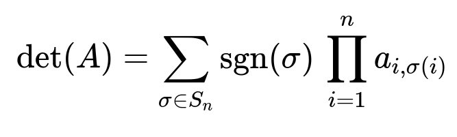
A is an n x n matrix with elements a_{i,j}.
S_n is the set of all permutations of {1, 2, ..., n}.
sigma is a specific permutation in S_n.
sgn(sigma) is the sign of the permutation sigma (+1 for even permutations, -1 for odd permutations).
a_{i, sigma(i)} is the element of the matrix in row i, column sigma(i).
This formula shows that the determinant is the sum over all possible ways of permuting columns of the matrix, each weighted by the sign of that permutation.
Cofactor Expansion (Laplace Expansion)
a_{i,j} is the element in row i, column j of matrix A.
A_{i,j} is the submatrix obtained by removing row i and column j from A.
(-1)^{i+j} is the factor that accounts for the sign associated with the cofactor of a_{i,j}.
The expression can be done along any row i or any column j (you pick i or j arbitrarily, typically whichever row or column looks easiest for computation).
This cofactor expansion formula is often used to compute determinants by hand, especially for matrices of moderate size (like 3 x 3 or 4 x 4).
Small Examples
For a 2 x 2 matrix:
[ a b ] [ c d ]
the determinant can be computed as (ad - bc).
For a 3 x 3 matrix, you can choose a row or column for expansion. As an example, expanding along the first row:
Let the matrix be: [ a11 a12 a13 ] [ a21 a22 a23 ] [ a31 a32 a33 ]
det(A) = a11 * (a22a33 - a23a32) - a12 * (a21a33 - a23a31) + a13 * (a21a32 - a22a31)
Computation in Practice
In practical numerical computation (e.g., in libraries like NumPy, PyTorch, or TensorFlow), the determinant is typically computed using transformations such as LU decomposition, which is more numerically stable. For an n x n matrix, these decomposition-based methods have a time complexity roughly O(n^3), which is more efficient than directly using the permutation formula (that would be O(n!) complexity).
Potential Follow-Up Questions
What makes the determinant zero and why does that imply the matrix is singular?
A matrix has a zero determinant if and only if its rows (or columns) are linearly dependent. Linear dependence means there is no unique way to solve the system of linear equations A*x = b for x if the determinant is zero, so the matrix cannot be inverted.
When rows or columns are linearly dependent, it effectively collapses the dimensional space that the matrix spans. Another intuitive way to see it is by relating the determinant to the “volume” scaling factor of the linear transformation described by the matrix. If the determinant is zero, the transformation flattens the space into a lower-dimensional subspace, eliminating any volume.
Why is the sign of the determinant important?
The determinant’s sign (+ or -) tells you how the orientation of the space is affected by the matrix transformation. A positive determinant indicates the transformation preserves the orientation of the basis vectors, while a negative determinant indicates a flip (like a mirror reflection) in orientation.
How do floating-point errors affect determinant computation in large matrices?
When dealing with large or ill-conditioned matrices, floating-point round-off can accumulate and significantly impact the accuracy of the computed determinant. Numerical algorithms like LU decomposition still manage floating-point errors more gracefully compared to naive cofactor expansion, but for very large matrices, the determinant can become extremely large or small, leading to overflow or underflow in standard double-precision arithmetic.
Techniques to mitigate these errors include:
Using higher-precision data types (like 64-bit float or even arbitrary precision libraries if needed).
Employing pivoting strategies in decompositions (partial or complete pivoting with LU).
Scaling approaches to keep intermediate values within a reasonable numerical range.
How does row or column operations influence the determinant?
Swapping two rows (or two columns) multiplies the determinant by -1.
Multiplying a row (or column) by a scalar k multiplies the determinant by k.
Adding a multiple of one row to another row does not change the determinant.
These properties allow you to keep track of how row/column operations, used in matrix decompositions, affect the determinant.
Can the determinant be related to eigenvalues?
Yes. For an n x n matrix A, the product of its eigenvalues (counted with their algebraic multiplicities) is equal to det(A). If any eigenvalue is zero, the determinant is zero, and the matrix is singular.
How would you compute the determinant in code for a matrix in Python?
In practice, one would rarely implement the determinant from scratch except for educational purposes. Libraries provide optimized, stable routines. For example, using NumPy:
import numpy as np

A = np.array([[2, 5],
              [1, 3]], dtype=float)
detA = np.linalg.det(A)
print(detA)  # Output: 1.0 (approximately)
Under the hood, NumPy’s linalg.det function uses LU decomposition (or a similar factorization) to compute the determinant efficiently and with better numerical stability compared to the naive definition.
By understanding both the theoretical definition and practical implementation details, you gain a thorough perspective on how and why determinants are computed.