
ML Interview Q Series: Explain, using mathematical reasoning, why Stochastic Gradient Descent is faster than full-batch Gradient Descent.

📚 Browse the full ML Interview series here.
Comprehensive Explanation
Stochastic Gradient Descent (often referred to simply as SGD) updates the model parameters using a single training example (or a small subset, known as a mini-batch) at each iteration, rather than computing the gradient using the entire training set. The fundamental reason SGD achieves speed gains is that it avoids the expensive full-batch gradient computation on every step and instead uses an estimate of the gradient based on fewer samples. Standard Gradient Descent (batch gradient descent) requires processing the entire dataset to compute each parameter update.
The traditional full-batch gradient descent updates parameters by computing a gradient over all N data points:

Here, theta_{t+1} is the updated parameter vector, theta_{t} is the current parameter vector, eta is the learning rate, L() is the loss function for a single training example, x_i and y_i represent the i-th data sample and its corresponding label, and N is the total number of training examples.
By contrast, SGD updates parameters by computing the gradient using only one sample (or a small mini-batch) at each iteration:
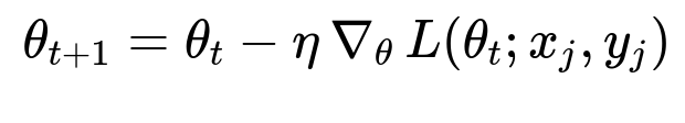
Here, x_j and y_j denote a randomly chosen single sample (or a small subset) from the dataset. Because the update relies on just one sample (or a few samples), the computation per iteration is much cheaper. Even though the gradient estimate is noisier than the full-batch gradient, in many practical settings this noisy gradient still points in a direction that generally decreases the loss.
Processing time for each iteration in standard gradient descent scales with N, because all data points must be processed before each update. In SGD, one iteration only processes a single (or a small fraction) of the data, making each parameter update significantly faster. Over many updates, SGD can converge more quickly in wall-clock time, especially when N is large.
This explains why SGD is computationally efficient: each step requires far fewer arithmetic operations than standard gradient descent. Although there may be more parameter updates overall, the total time to reach a reasonable region of the parameter space is often shorter.
Implementation Perspective
Below is a rough illustration of how one might implement standard gradient descent compared to stochastic gradient descent in Python. Notice that the main structural difference is that standard gradient descent computes the gradient over the entire dataset before a single update, while SGD computes and applies many individual (or mini-batch) updates throughout an epoch.
# Pseudocode for full-batch Gradient Descent
def full_batch_gradient_descent(X, y, theta, alpha, num_epochs):
    # X is the entire dataset, y are labels, theta are parameters
    # alpha is learning rate
    # num_epochs is the total number of passes over the data

    for epoch in range(num_epochs):
        # Compute gradient over the entire dataset
        gradient = compute_full_gradient(X, y, theta)

        # Update theta
        theta = theta - alpha * gradient

    return theta

# Pseudocode for Stochastic Gradient Descent
def stochastic_gradient_descent(X, y, theta, alpha, num_epochs):
    # For simplicity, assume X, y are arrays of length N
    N = len(X)

    for epoch in range(num_epochs):
        for i in range(N):
            # Pick one sample (x_i, y_i)
            # Or for mini-batch, pick a small subset
            x_i = X[i]
            y_i = y[i]

            # Compute gradient based on a single sample
            grad_i = compute_gradient_single_sample(x_i, y_i, theta)

            # Update theta
            theta = theta - alpha * grad_i

    return theta
Potential Convergence Behavior
Although SGD computes noisy gradients, it can still converge to regions near the global minimum when using appropriate techniques like learning rate decay or momentum-based optimizers. In high-dimensional problems or massive datasets, the computational advantage of SGD (or mini-batch SGD) typically outweighs the reduced accuracy of its gradient estimates at each step.
Follow-up Questions
How do we choose between full-batch Gradient Descent, Stochastic Gradient Descent, or Mini-Batch Gradient Descent in practice?
Choosing depends on factors like dataset size, hardware constraints, and training stability. With a very large dataset, full-batch gradient descent becomes prohibitively expensive per iteration. Stochastic gradient descent or mini-batch SGD is usually preferred because smaller batches fit into memory and allow more frequent updates. Full-batch methods can sometimes be useful for smaller datasets where computation is not as expensive, but in real-world scenarios with large data, mini-batch SGD is almost always the default approach.
How does mini-batch size influence training speed and convergence?
A mini-batch size that is too large may lead to slower per-iteration processing time, similar to full-batch methods. If the mini-batch is too small, the gradient estimates can become very noisy, potentially requiring more total iterations to converge. There is often a balance point where the mini-batch is large enough to produce stable gradient estimates but small enough to take advantage of efficient computations on modern hardware (such as GPUs). This balance point often needs empirical tuning.
Does SGD guarantee convergence to the global minimum?
For convex problems (such as simple linear regression with a convex loss), SGD can theoretically converge to the global minimum, though it may require carefully chosen learning rate schedules. For non-convex problems such as deep neural network training, SGD typically converges to a local minimum or a saddle point region. However, these local minima often generalize well for many deep learning tasks. Proper strategies like momentum, adaptive learning rates, or weight decay can help smooth out the noise and achieve better convergence.
Why is a random order of samples important in SGD?
If the samples are processed in a fixed order that might have some underlying pattern, the gradient updates could become biased toward certain directions. Shuffling the dataset each epoch ensures the gradient noise is more uniformly random. This typically produces better, more stable convergence behavior.
What happens if the dataset is extremely small? Is SGD still beneficial?
When the dataset is small, a full-batch approach is often feasible because the computational cost of processing the entire dataset is not large. In this situation, the difference in time between full-batch gradient descent and stochastic approaches is minimal. Additionally, the gradient of the entire dataset might be more reliable, so full-batch gradient descent can converge smoothly. Nevertheless, if the dataset is not tiny but is moderately sized, mini-batch methods still offer a good trade-off between gradient accuracy and computational speed.
Are there any pitfalls regarding learning rates when switching from full-batch to SGD?
When using SGD, a static learning rate can cause large oscillations if it is not set properly. A common approach is to use a higher initial learning rate compared to full-batch methods and then decay it over time. Techniques like exponential decay, step decay, or more advanced optimizers (e.g., Adam, RMSProp) are frequently used to manage and adapt the learning rate during training. A poorly tuned learning rate can hamper or prevent convergence for SGD.
Summary of Key Points
Stochastic Gradient Descent accelerates training time compared to standard full-batch Gradient Descent by computing an approximate gradient on subsets of data. Although each update is less exact, the massive reduction in per-iteration compute often leads to faster overall convergence in practice. Proper learning rate schedules, careful mini-batch size selection, and randomization all influence SGD’s effectiveness and stability in both convex and non-convex optimization problems.
Below are additional follow-up questions
How does the variance in the gradient estimate under SGD affect convergence?
When using only one sample (or a small batch) to compute the gradient, there is an inherent variance because that single sample may not accurately represent the entire dataset. This variance typically manifests as noisy parameter updates. Sometimes, these updates can overshoot or deviate from the “true” gradient direction one would obtain with a full-batch approach. Despite this randomness, the gradient over many updates tends to average out. As long as the learning rate is managed properly—often decaying over time—the noisy steps can still converge effectively. However, if the learning rate is not decayed or is too large, the high variance can cause prolonged oscillations or even divergence.
Potential pitfall:
If the variance is too large and the learning rate remains constant, the parameters might bounce around, never settling into a minimum. This typically leads to either a plateau in performance or outright failure to converge.
Why might one apply momentum-based or adaptive optimization methods (e.g., Adam) to SGD?
Momentum-based or adaptive methods tackle the issue of noise and oscillation by accumulating historical gradient information. Momentum smooths out updates by effectively applying a moving average to the gradients; Adam, RMSProp, and other adaptive methods adjust the learning rate of each parameter individually based on past gradients.
Momentum advantage:
Faster and smoother convergence in directions with consistent gradients.
Mitigates the zigzag phenomenon in regions with steep curvature.
Adaptive advantage:
Adjusts learning rates automatically, allowing different parameters to progress at different speeds.
Helps maintain stability when certain parameters are updated frequently with large gradient magnitudes.
Potential pitfall:
Over-reliance on momentum or adaptive updates can sometimes miss the best local region if the optimizer overshoots. Carefully tuning hyperparameters (learning rate, momentum terms, betas in Adam) remains crucial.
How does distributed training interact with SGD's efficiency?
In large-scale training, data is often split across many machines or GPUs. Each node can perform SGD steps on its subset of data (or mini-batches) and then synchronize parameter updates. Although this parallelization leads to speedups, one must manage communication overhead carefully. If synchronization is too frequent or handled inefficiently, the computational speed advantage of parallelized SGD can be diminished by network delays or the cost of combining gradients.
Potential pitfall:
Inconsistent updates arise when different nodes are out of sync. Techniques like asynchronous SGD can reduce waiting times but at the cost of stale gradient updates. Using techniques such as ring-allreduce or parameter servers can strike a balance between throughput and update freshness.
What if the data distribution shifts over time (concept drift)? How does SGD perform?
If the underlying data distribution changes, as might happen in real-time applications (e.g., user behavior in online systems), the loss landscape can shift. SGD is generally more responsive to such changes than full-batch gradient descent because it updates parameters frequently. Each new batch effectively adapts the model to the most recent data distribution.
Potential pitfall:
Excessive noise or rapid changes can lead to perpetual updates that overfit to the most recent samples. A well-structured strategy—like applying a rolling window of data, decaying older samples, or adjusting the learning rate over time—often becomes necessary.
Does SGD handle outliers better than full-batch gradient descent?
Outliers can exert a strong influence when computing a single gradient based on the entire dataset. In SGD, each outlier might only sporadically affect a single step. Over multiple updates, the impact of outliers can be “diluted” compared to the consistent gradient contribution they exert in full-batch methods. However, this is not an absolute solution—extreme outliers can still cause occasional large gradient steps in SGD.
Potential pitfall:
If outliers appear repeatedly or if there is a substantial fraction of outliers, SGD might be pulled away from good solutions. Robust loss functions or data pre-processing techniques become necessary to mitigate outlier effects in such cases.
How does SGD behave in extremely noisy objective landscapes?
When the objective function itself has a high level of inherent noise (common in scenarios like reinforcement learning, where the reward signal is unstable), the gradient is already uncertain. SGD’s own noise adds to this uncertainty. Nonetheless, the frequent updates in SGD help the model adapt more dynamically. Properly tuned hyperparameters, such as a decaying or smaller learning rate, can help the model avoid getting lost in the noise.
Potential pitfall:
If the environment noise and gradient noise combine, the model can bounce erratically. This may require advanced techniques like reward shaping, state-space smoothing, or specialized exploration strategies to provide more stable learning signals.
When should we consider averaging model parameters during SGD (e.g., Polyak or SWA)?
Parameter averaging, such as Polyak averaging, involves keeping a running average of past parameter states to smooth out the noise from individual updates. Stochastic Weight Averaging (SWA) extends this concept in a practical manner by periodically recording parameters during later epochs, then averaging them to produce a final model.
Potential advantage:
This can reduce variance in the final parameters, often improving generalization or smoothing the final solution landscape.
Potential pitfall:
If the model is still in the rapid-learning phase (high gradient magnitude, large updates), averaging might smear out useful, direction-setting updates. Averaging is typically most beneficial when the model’s updates have slowed and it is oscillating around a neighborhood of good solutions.
What sampling strategies exist for SGD, and do they matter?
Common approaches:
Shuffle each epoch. Each pass (epoch) involves shuffling the entire dataset, processing it in mini-batches in random order.
Reservoir or streaming sampling. If the dataset is extremely large or continuously generated, one might use streaming methods to maintain a representative sample in memory.
Potential advantage:
Shuffling data each epoch reduces correlation between consecutive samples. This typically provides more stable gradient updates.
Potential pitfall:
If the data has structure (e.g., sorted by label or time), not shuffling can skew the gradient updates. Randomization overhead might be non-trivial for massive datasets, so one must balance perfect shuffling with memory and time constraints.
How does SGD fare with correlated samples (e.g., in reinforcement learning or time series)?
SGD assumes that samples are drawn independently. In reinforcement learning or time series, consecutive states can be highly correlated. This correlation reduces the effective variance advantage of random sampling and can create strong biases in updates. Techniques like replay buffers, skip sampling, or decorrelation procedures are often employed to reintroduce some level of independence in samples.
Potential pitfall:
If one directly uses SGD on sequentially correlated data, the training signal can consistently push the model in a particular direction, ignoring other important parts of the state space. This often leads to suboptimal convergence or overfitting to a narrow slice of time steps.
How do we implement SGD on huge datasets that do not fit into memory?
In scenarios where even storing the dataset in memory is infeasible, one can stream data from disk in small batches (online learning style). At each step, only a small portion of data is loaded, processed, and used for parameter updates. Tools like generators in Python or specialized frameworks that handle large datasets (e.g., Apache Spark, Dask, or TensorFlow Dataset) facilitate out-of-core learning.
Potential pitfall:
I/O bottlenecks can slow down training if data loading and model updates are not properly parallelized. One might need to buffer multiple batches in memory or use prefetching and caching mechanisms to ensure that the computation pipeline remains fed with data.