ML Interview Q Series: Explain what is Cost (Loss) Function in Machine Learning?

📚 Browse the full ML Interview series here.

Comprehensive Explanation

A cost function, also known as a loss function, is a mathematical formulation that measures how far off a model’s predictions are from the actual target labels. In other words, it quantifies the “cost” or “penalty” incurred for making poor predictions. By minimizing the cost function, we can guide the training process to adjust the model's parameters toward more accurate predictions.

A simple example in regression tasks is the mean squared error (MSE) cost function. This function calculates the average of the squares of the differences between the predicted values and the actual values. Minimizing it forces the model to reduce large errors more aggressively.

Core Mathematical Example (MSE for Linear Regression)

Below is the MSE cost function for a regression setting in h1 font (as per instructions):

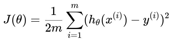
Here, J(\theta) is the cost function with respect to the model parameters theta. The summation runs from i=1 to i=m, where m is the total number of training examples. For each training example, x^(i) is the input feature vector, h_theta(x^(i)) is the model’s prediction, and y^(i) is the actual label for that example. We include 1/(2m) for convenience, so the derivative becomes simpler (the 2 cancels out when we differentiate).

After computing this cost function, optimization algorithms (for example, gradient descent) adjust the parameters theta to minimize J(theta) by iteratively moving in the direction of negative gradients.

Other Common Loss Functions in Machine Learning

For classification tasks, people often use cross-entropy loss (also known as log loss). In plain text, for a binary classification task with predicted probability p for the positive class and ground truth label y in {0,1}, the cross-entropy loss might look like:

Minimizing it encourages the model to output probabilities closer to 1 for the correct class, while heavily penalizing confident but wrong predictions.

For multi-class classification tasks, cross-entropy can be extended using a summation across all classes, so each instance’s loss accounts for the log of the predicted probability of the true class.

Why Cost Functions are Crucial

They provide a quantifiable and differentiable objective. By computing its gradient (slope), optimization methods know how to update the model’s parameters to improve predictions. This feedback loop — comparing predicted output versus actual output, computing cost, and adjusting parameters — is fundamental to training neural networks and other ML models.

Impact of Different Cost Functions

Using different cost functions can shift a model’s behavior. For instance, mean absolute error focuses on absolute deviations, making the model less sensitive to outliers than mean squared error. Cross-entropy directly corresponds to maximizing likelihood in classification, so it’s naturally aligned with probabilistic interpretations. The choice of loss function often depends on domain requirements, data distribution, and performance objectives.

Follow-up Questions

Could you explain how the gradient descent algorithm uses the cost function?

Gradient descent updates parameters in the direction that locally minimizes the cost function. First, compute partial derivatives (gradients) of the cost function with respect to each model parameter. Then subtract a fraction (learning rate) of that gradient from the parameter value. This process is repeated for many iterations (epochs), gradually moving theta toward a local minimum. The cost function serves as a “landscape,” and gradient descent tries to find the point where that landscape is lowest.

Are there scenarios where we might modify the cost function?

Yes, there are many scenarios where we modify or augment the cost function:

We can add regularization terms to penalize large parameter values (L2 or L1) to address overfitting. In this case, the cost function might have an additional term like alpha * sum(theta_j^2) or alpha * sum(abs(theta_j)), where alpha is a hyperparameter controlling the strength of regularization.

We can have cost-sensitive learning in classification when one type of misclassification is more expensive than another (for example, in medical diagnosis, missing a positive case might be more costly than a false alarm).

We can incorporate custom penalty terms for domain-specific constraints, such as making sure certain features or constraints remain within particular ranges.

How do we handle imbalanced data in the cost function?

In highly imbalanced classification tasks, standard cost functions like standard cross-entropy might not be enough, because the model can exploit class imbalance to achieve high accuracy by mostly predicting the majority class. Some strategies include:

Weighting the loss function so that mistakes on the minority class receive higher penalty. For instance, the cross-entropy loss can be multiplied by a class weight that re-balances classes.

Using focal loss, which is a modified form of cross-entropy that reduces the relative loss for well-classified examples, focusing more on hard misclassified examples.

Using data-level approaches like oversampling the minority class or undersampling the majority class to provide a more balanced training distribution.

How can we implement a simple custom cost function in PyTorch?

Below is a minimal Python code snippet illustrating how to create a custom mean absolute error (MAE) cost function in PyTorch:

import torch
import torch.nn as nn

class CustomMAELoss(nn.Module):
    def __init__(self):
        super(CustomMAELoss, self).__init__()

    def forward(self, predictions, targets):
        # predictions and targets are assumed to be torch tensors
        # with the same shape
        # This computes mean absolute error
        loss = torch.mean(torch.abs(predictions - targets))
        return loss

# Example usage
preds = torch.tensor([2.0, 3.0, 4.0])
labels = torch.tensor([1.0, 3.5, 5.0])
criterion = CustomMAELoss()
cost = criterion(preds, labels)
print(cost.item())

This code snippet defines a subclass of nn.Module to hold the forward computation of the MAE loss. In practice, you could similarly implement other cost functions. PyTorch also provides many built-in loss functions like nn.MSELoss, nn.BCELoss, nn.CrossEntropyLoss, and nn.NLLLoss for convenience.

What happens if the cost function is not differentiable?

Many optimization routines rely on gradient-based methods, requiring a differentiable cost function. If the cost function has points of non-differentiability (for example, absolute value at zero), subgradient or specialized optimization approaches might be used. Techniques like approximate smoothing or switching to a surrogate loss are common.

Additionally, some frameworks allow gradient-free optimization approaches, or they can handle piecewise derivatives (like ReLU for neural networks).

How do we select an appropriate cost function?

The choice often depends on:

The problem type (regression vs. classification vs. ranking vs. other tasks).

The data distribution and presence of outliers or class imbalance.

The desired interpretation: Are probabilities critical, or is direct numeric distance more important?

The computational convenience: Some cost functions have nicer derivatives and lead to simpler optimization steps.

Balancing these factors is key, and often you might experiment with multiple loss functions or incorporate domain knowledge to decide which cost function aligns best with the real-world objectives.

Below are additional follow-up questions

How can we interpret the scale of cost function values across different tasks?

Different machine learning tasks often have cost functions that naturally vary in magnitude. For example, mean squared error (MSE) in regression could be much larger in tasks involving large target values (like predicting house prices) compared to tasks where targets range between 0 and 1. Cross-entropy loss for classification is typically within a narrower range, often between 0 and a small positive value. Because these scales differ, comparing cost function values across tasks directly is usually meaningless. It is more relevant to compare the decrease in the cost function over time for the same task or to track relative improvements. One potential pitfall is automatically selecting hyperparameters (like learning rate) based on absolute cost function scales without normalizing them. This could lead to very slow or unstable training.

What if the cost function is poorly scaled? How does that impact training?

If the cost function produces very large values, gradient-based methods might compute huge gradients, potentially causing erratic parameter updates and making training unstable. Conversely, if the cost function is extremely small, gradient updates might be tiny, slowing convergence dramatically. To address such scaling issues, we can:

• Normalize or standardize input features so that the cost function has more consistent magnitudes of partial derivatives. • Use adaptive learning rate optimizers like Adam or RMSProp that self-adjust parameter update scales. • Apply transformations (like dividing by a constant factor) to the cost function or to its constituent terms to ensure that its values are within a reasonable range.

A real-world subtlety arises in multi-loss scenarios, where you may have multiple objectives contributing to a combined cost. If one of them is naturally larger in scale, it might dominate training, overshadowing other objectives.

How does cost function design differ in unsupervised learning or reinforcement learning?

In unsupervised learning, we often do not have explicit labels. Instead, we might minimize reconstruction error (as in autoencoders) or maximize likelihood of observed data (as in probabilistic clustering). For autoencoders, the cost function might be something like the MSE between the input and the reconstructed input, or it might be a cross-entropy loss in the case of binary inputs. The lack of ground truth labels means the cost function must capture the inherent structure of the data itself. A pitfall here is that the model can learn trivial solutions (e.g., copying inputs in autoencoders without learning meaningful latent structure).

In reinforcement learning, the concept of a “cost” or “reward” is more long-term. The objective might be to maximize cumulative reward rather than simply matching a target. Value-based methods define a cost function that measures the difference between current value estimates and discounted future rewards. One subtlety is that noisy or sparse reward signals can make it difficult to propagate meaningful gradient information to the model. Moreover, reward shaping can drastically alter learning behavior, and incorrectly designed reward signals can lead to unintended or even adversarial policies.

How does the cost function shape model convergence in neural networks versus simpler models like linear regression?

In linear regression, convex cost functions (like MSE) guarantee a single global minimum. Gradient descent or analytical solutions can find that optimum systematically. In neural networks, cost functions are typically non-convex due to complex architectures and non-linearities. Consequently, we might encounter many local minima, saddle points, or flat regions. The optimization can become more involved, and different initializations or hyperparameters might yield different local minima. Cost function design in neural networks can encourage or discourage certain behaviors — for instance, using a margin-based loss (like hinge loss in SVMs) can encourage robust classification boundaries. In practice, advanced optimizers (e.g., Adam) and regularization techniques (e.g., dropout) are often used to help navigate this high-dimensional, non-convex cost landscape.

When do we prefer Huber loss or L1 loss over MSE in regression tasks, and what are potential pitfalls?

MSE penalizes large errors more severely, which can be problematic if outliers exist; the model might over-adjust to a small number of extreme points. L1 loss (absolute error) is more robust to outliers but is not differentiable at zero, which can complicate gradient-based updates (though frameworks typically handle this via subgradient or a small smoothing). Huber loss is a compromise: it behaves like MSE near small errors and L1 for large errors. This means moderate deviations get punished quadratically, while huge deviations do not overpower the training. A subtle pitfall is that if you expect truly large outliers in your data, even Huber might not sufficiently down-weight them; sometimes specialized robust loss functions are preferred. Another pitfall is that switching from MSE to L1 can change the distribution of errors you converge to (L1 solutions often favor median-like fitting).

What is the difference between training loss and validation loss, and how do we interpret them for overfitting or underfitting?

Training loss is computed on the same data used to adjust the model’s parameters, so it tends to decrease steadily as the model fits that data more closely. Validation loss is measured on a separate held-out set, serving as a proxy for how well the model generalizes to unseen data. If training loss is much lower than validation loss, that signals overfitting — the model is memorizing patterns that do not generalize. If both training and validation losses are high, the model might be underfitting, indicating insufficient complexity or suboptimal hyperparameters. By monitoring these losses in tandem, we can decide when to apply regularization, gather more data, or adjust learning rates. A subtlety arises with time series or streaming data, where the validation set might shift in distribution over time; in such cases, evaluating “out-of-distribution” validation can be misleading if future data differ significantly.

How do cost functions adapt to real-time or online learning scenarios?

In online learning, data arrives in sequential fashion, and the model updates continuously. Traditional batch-based cost functions accumulate gradients over entire datasets, which may be impractical in a streaming scenario. Instead, we compute incremental or mini-batch updates. This means our cost function at each step might be just the error on the newly arrived data or a small chunk of data. A pitfall here is the potential for large variance in parameter updates if the new data is not representative. Also, concept drift can occur in dynamic environments — the cost function remains the same, but the distribution of data might shift. Hence, the model must adapt by continually updating parameters and possibly adjusting hyperparameters like learning rate. Another subtlety is balancing stability (not forgetting old knowledge) with plasticity (adapting to new patterns) in the cost function’s optimization.

In practice, how do we debug a situation where the cost function does not go down during training?

If the cost remains the same or decreases very slowly, it could be due to:

• Learning rate issues: Too high can cause divergence or oscillation, too low can stall progress. • Incorrect computation graph: For instance, forgetting to zero out gradients between mini-batches in PyTorch. • Dead neurons or vanishing/exploding gradients: In deep networks, certain activation functions or weight initializations can exacerbate these issues. • Data preprocessing errors: If data has not been scaled or normalized properly, large gradient steps might hamper learning. • Implementation bugs: For instance, mixing up predictions and labels or incorrectly calculating the loss.

A real-world subtlety is that if the cost is not decreasing, but your evaluation metrics are improving, it might mean your cost function is not aligned with your actual performance metric. Or it could mean something is off in how you are logging and visualizing the cost.

Why might we use more than one cost function at once?

Sometimes we have multiple, potentially conflicting objectives. For example, in multi-task learning, we might simultaneously want a model to perform classification and regression. In these scenarios, the overall cost is often a weighted sum of individual cost functions. A key subtlety is choosing the right weighting: If one cost dominates numerically, it can overshadow other tasks. Another subtlety is that these tasks might share some underlying representation but diverge in how best to train them (e.g., classification might prefer cross-entropy, while regression might prefer MSE). Balancing them requires domain insight or systematic hyperparameter tuning to get synergy across the tasks instead of diluting performance on each.

Can a cost function lead to biased or unfair outcomes, and how might we address that?

Yes. If the cost function focuses solely on overall accuracy or cross-entropy, the model may systematically discriminate against underrepresented groups, especially in imbalanced or sensitive domains. For example, if the training data is skewed, the model might learn patterns that exacerbate societal biases. To address fairness concerns, we can introduce fairness-driven modifications to the cost function, like penalizing large performance gaps between demographic groups or adding constraints for demographic parity or equal opportunity. A subtlety is that addressing bias with cost function adjustments can trade off overall performance. Another pitfall is incomplete or faulty fairness metrics that might not capture real-world complexity. When introducing fairness-driven terms, it is essential to evaluate on multiple fairness criteria and ensure we are not shifting bias to other subgroups inadvertently.