
ML Interview Q Series: Explain what characterizes a function as convex. Then provide a concrete example of a non-convex machine learning algorithm and clarify why it is non-convex.
📚 Browse the full ML Interview series here.
Short Compact solution


always lies above (or touches) the function curve. One key property of a convex function is that any local minimum is also a global minimum.
Neural networks are a classic illustration of non-convexity in machine learning. Since neural networks can approximate a wide range of complex functions (many of which are non-convex), their cost landscape generally has multiple local minima and saddle points. Furthermore, swapping parameters across different neurons can yield the same output while altering the cost surface, thus leading to many local optima. For these reasons, neural network cost functions are inherently non-convex.
Comprehensive Explanation
What Is Convexity?

This condition implies that the function’s slope never “bends downwards” in a way that would create multiple distinct local minima. Consequently, one of the most important attributes of convex functions is that local minima are also global minima. In optimization scenarios, this property greatly simplifies finding the global optimum because any method that converges to a stationary point will effectively find the global solution.
Why Convexity Matters in Machine Learning
From a machine learning standpoint, especially when training models, optimization typically involves minimizing some loss (cost) function. If the loss function were convex in the parameters we are optimizing, we would have guarantees about finding the global optimum (given a suitable optimization algorithm). Classic examples include:
Linear Regression with a Mean-Squared Error (MSE) loss: The cost function is convex in the weights.
Logistic Regression: With an appropriate regularization term, the loss is typically convex in the parameters.
Convex cost functions mean fewer headaches when searching for global minima; however, most interesting modern models—such as deep neural networks—depart from convexity to achieve richer representational power.
Example of a Non-Convex Algorithm: Neural Networks
Neural networks serve as a primary example of models with non-convex objective functions. The universal approximation capability allows these networks to represent extremely flexible mappings from inputs to outputs. The result of having such a flexible architecture (with many parameters interacting in highly nonlinear ways) is that:
Multiple Local Minima: The error (loss) surface often contains numerous local minima. While recent research suggests that many of these local minima often perform similarly in terms of generalization, they still complicate the theoretical analysis.
Parameter Symmetries: If you swap the parameters of two neurons within the same layer, the overall function might remain identical, but you effectively find a different point in parameter space, which could be interpreted as a different local minimum in the cost landscape.
Saddle Points and Flat Regions: The high-dimensional parameter space is filled with saddle points and regions where gradients can be very small, complicating training and possibly requiring advanced optimization strategies or heuristics (like learning rate schedules, momentum, or adaptive gradient methods).
Hence, neural networks are textbook examples of non-convex cost surfaces in machine learning.
Practical Consequences and Strategies
Local Minima vs. Global Minima: In non-convex settings, finding a “true” global minimum is typically infeasible. However, empirically, in deep learning, we often discover parameters that achieve good performance in practice, even if they are not globally optimal.
Initialization: Because of the complex loss surface, a model’s final parameters can depend heavily on the initialization strategy. This explains why careful initialization (e.g., Xavier or Kaiming initialization) can significantly impact training success.
Regularization and Architecture: Certain architectures or regularization methods can smooth out the error surface, potentially reducing the number and severity of suboptimal local minima or saddle points.
Below is a small PyTorch code snippet that illustrates a very simple neural network that has a non-convex loss surface. The code is not meant to show a guaranteed local minimum trap, but rather to highlight the structure of an MLP with nonlinear activations that inherently leads to a non-convex optimization problem:
import torch
import torch.nn as nn
import torch.optim as optim

# Simple feedforward network
class SimpleMLP(nn.Module):
    def __init__(self, input_dim, hidden_dim, output_dim):
        super(SimpleMLP, self).__init__()
        self.fc1 = nn.Linear(input_dim, hidden_dim)
        self.relu = nn.ReLU()
        self.fc2 = nn.Linear(hidden_dim, output_dim)

    def forward(self, x):
        x = self.fc1(x)
        x = self.relu(x)
        x = self.fc2(x)
        return x

# Example usage
model = SimpleMLP(input_dim=10, hidden_dim=5, output_dim=1)
criterion = nn.MSELoss()
optimizer = optim.SGD(model.parameters(), lr=0.01)

# Dummy data
inputs = torch.randn(32, 10)
targets = torch.randn(32, 1)

# One training step
optimizer.zero_grad()
outputs = model(inputs)
loss = criterion(outputs, targets)
loss.backward()
optimizer.step()
Although this snippet may converge toward some solution that minimizes the MSE loss, there is no guarantee (unlike a purely convex problem) that the found solution is globally optimal. In practice, many local minima or saddle regions might produce similar levels of performance.
Possible Follow-Up Questions
How does convexity or non-convexity influence the optimization process?
A convex objective guarantees that any local minimum is a global minimum. This can simplify the choice of optimization algorithm, since gradient-based techniques (like gradient descent) will converge to the global optimum under mild conditions. In non-convex problems, gradient-based methods can get stuck in local minima or saddle points, and different initializations or hyperparameters can produce different final solutions. Despite these challenges, empirical evidence shows that for large neural networks, many local minima often generalize similarly, making non-convexity less of a practical barrier than one might fear in theory.
What is the difference between convex and strongly convex functions?
While a convex function satisfies
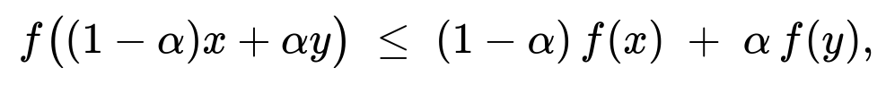
a strongly convex function imposes an additional condition that it is bounded away from linear combinations by a strictly positive factor. In simpler terms, strongly convex functions “curve upwards” more aggressively. Optimization of strongly convex functions is even more straightforward because it ensures unique global minima and faster convergence rates for gradient-based methods.
Why do neural networks inherently rely on non-convex cost functions?
Neural networks use compositions of linear transformations and nonlinear activations. The moment a nonlinear activation (like ReLU, sigmoid, or tanh) is introduced, the resulting function from inputs to outputs becomes non-convex in the model parameters. The universal approximation property requires these nonlinearities—without them, the network could not represent sufficiently complex functions. Thus, the flexibility that deep networks provide inherently comes at the cost of a non-convex optimization landscape.
Can we still train neural networks effectively if their cost function is not convex?
Yes. Despite the theoretical complications, in practice, we have developed numerous techniques—such as sophisticated weight initialization methods, batch normalization, adaptive optimizers (Adam, RMSProp), momentum, learning rate schedules, and various forms of regularization—that help the optimization process navigate non-convex landscapes. Furthermore, modern neural networks often have very high-dimensional parameter spaces, where local minima can sometimes be “shallow” and not drastically different in terms of performance. Empirical evidence suggests that these methods often converge to parameter configurations with excellent generalization properties.
How do we reduce or mitigate the effect of local minima in neural networks?
Good Initialization: Proper initialization can help the model start in a region of parameter space less prone to poor local minima.
Regularization and Architecture Choices: Structural choices (like skip connections in residual networks) can smooth out the loss landscape and help the network train more reliably.
Stochastic Optimization: Stochastic gradient descent or mini-batch training inherently introduces noise that can help escape certain local traps.
Ensemble Methods: Training multiple neural networks with different initializations and averaging predictions can hedge against getting stuck in any particular bad local minimum.
These strategies do not guarantee global optimality in a strict sense, but they frequently lead to solutions that work well in practical scenarios.
Below are additional follow-up questions
How do convex sets differ from convex functions, and why is this distinction important in optimization?

A convex function is about how a function’s value lies relative to straight lines drawn between two points on its graph. Although related, the two definitions address different parts of an optimization problem. Specifically:
Convex sets are important for defining feasible regions in constrained optimization. If the constraint set is convex, it is “friendly” for many optimization algorithms because there are no “holes” or “inward dents” in the feasible region.
Convex functions determine the shape of the objective (cost) function that must be minimized or maximized. A convex objective has the property that local minima are global minima.
Potential Pitfalls and Real-World Issues
When dealing with real-world constraints, one can inadvertently define a non-convex feasible region (e.g., a region that has multiple disjoint parts). Even if the objective function is convex, the overall problem might be non-convex because the feasible set is not convex.
In combinatorial optimization tasks (like feature selection with

constraints), the feasible set is often highly non-convex, making the problem extremely challenging despite any local convexity in the function itself.

How can second-order methods (like Newton’s method) help in convex vs. non-convex optimization, and what are their limitations?

In Convex Optimization
A positive semi-definite Hessian throughout the domain indicates convexity. When this is the case, Newton’s method converges extremely quickly (often in a small number of steps) if the Hessian is well-conditioned.
Convergence is guaranteed to a global minimum in convex problems, assuming you remain in the interior of the convex region.
In Non-Convex Optimization
The Hessian can have positive and negative eigenvalues, indicating saddle points or local maxima/minima. Newton’s method might converge to a local (rather than a global) optimum or get stuck in a saddle point.
Implementing second-order methods for large-scale neural networks (where parameter dimensions can be in the millions) is impractical: storing and inverting the Hessian is computationally infeasible.
Potential Pitfalls and Real-World Issues
Even quasi-Newton methods like BFGS, which approximate the Hessian, can still be too big to handle in many deep learning applications.
In non-convex settings, second-order information might not always accelerate convergence if the Hessian points toward a suboptimal region.
Numerical instability or ill-conditioning of the Hessian can cause large, erratic parameter updates, leading to divergence rather than convergence.
Why is it not always feasible to turn a non-convex neural network objective into a convex one by modifying the architecture or the loss function?
Neural networks rely on nonlinear activations (ReLU, sigmoid, tanh, etc.) to capture complex, highly non-linear relationships in data. If we replaced these activations or altered the network structure to enforce convexity in the parameters, we would severely limit the network’s expressiveness. For example:
Restricting a network to purely linear operations yields a model equivalent to linear regression, which is convex but has limited representational capacity.
Eliminating multi-layer depth or restricting activation functions to preserve convexity would undercut the universal approximation property of neural networks.
Potential Pitfalls and Real-World Issues
Certain special architectures (like convex neural architectures or kernel methods) can maintain convexity with respect to certain parameters, but they often involve trade-offs in flexibility or scale poorly to large problems.
Some researchers investigate “convex formulations of deep learning,” but these can be computationally very expensive or require assumptions that don’t hold in most real-world scenarios.
How do high-dimensional parameter spaces affect our understanding of local vs. global minima in non-convex problems?
In high dimensions (such as neural networks with millions of parameters), the notion of a “valley” or “local minimum” differs from low-dimensional intuition:
Saddle Points are often more prevalent than strict local minima in high-dimensional spaces. A saddle point in high dimensions might still trap gradient descent temporarily, but slight random perturbations or stochastic noise can help escape it.
There is a hypothesis that in very high dimensions, most local minima are “good” minima in the sense that they have similar loss values and generalization properties—this is sometimes referred to as the “wide minima” or “flat minima” phenomenon.
Potential Pitfalls and Real-World Issues
High-dimensional geometry can be counterintuitive. For example, distance metrics (e.g., Euclidean) behave differently, and small regions may have surprisingly large volumes in high-dimensional spaces.
Empirically, a solution that is a local minimum in one cross-section of parameter space might effectively be a saddle region in another cross-section, confusing typical low-dimensional diagnostic methods.
What is the role of curriculum learning in navigating non-convex loss landscapes?
Curriculum learning involves training models by presenting simpler examples or tasks first, then gradually increasing complexity. The underlying idea is that the model parameters evolve in a smoother region of the parameter space before tackling harder examples, potentially avoiding poorly generalizing minima early in training.
Initialization Sensitivity: By starting with easier tasks, the model’s initial parameters may be guided into more favorable basins of attraction in the loss landscape.
Gradual Complexity: When tasks become progressively more difficult, the model adjusts parameters in smaller, more controlled steps, potentially reducing the risk of abrupt divergences.
Potential Pitfalls and Real-World Issues
Curriculum strategies may overconstrain the model or cause it to overfit to simpler tasks if not managed carefully (e.g., ensuring that the “easy tasks” are still representative of the final data distribution).
Determining the correct “order” or “pace” of difficulty levels is highly problem-specific and can require trial and error or domain expertise.
How does overparameterization in deep neural networks influence the landscape of local minima?
Overparameterization refers to having far more parameters than the minimum needed to fit the data. Modern deep networks often have millions (or even billions) of parameters:
Empirical Evidence: Overparameterized networks can achieve very low training error, sometimes even zero, indicating that the optimization can find solutions that fit the training set perfectly.
Landscape Flattening: Having so many parameters can create a landscape with many wide, flat minima where different parameter configurations lead to similar performance. This can paradoxically make optimization simpler because the network is less likely to get “stuck” in deep, narrow local minima.
Potential Pitfalls and Real-World Issues
Overfitting: Overparameterization can lead to memorizing training data, potentially harming generalization if not controlled with techniques like early stopping, regularization, or large-scale data augmentation.
Generalization Mystery: It remains somewhat puzzling why, in many practical cases, overparameterized models generalize well despite having the capacity to overfit. This is an active area of theoretical research and can appear contradictory to classical learning theory.
When might non-convex solutions be preferable to convex ones in a real-world ML project?
Although convex solutions are more predictable and theoretically reassuring, they can be insufficient for capturing the intricacies of many real-world data distributions or complex relationships in high-dimensional data:
Complex Feature Interactions: In tasks such as image recognition or language modeling, interactions among features are often highly nonlinear, which a convex model (like a simple linear classifier) cannot adequately capture.
Computational Constraints: Certain convex methods (e.g., large-scale quadratic programming) might become computationally intractable for extremely large datasets, whereas heuristics for non-convex deep learning can scale efficiently with GPUs.
Potential Pitfalls and Real-World Issues
When using a non-convex model, one must be cautious about hyperparameter tuning, data preprocessing, and initialization, as they significantly affect the final solution.
In critical applications (e.g., medical diagnostics, finance), the unpredictability of training outcomes in non-convex models might necessitate additional testing or interpretability strategies, increasing both development time and computational cost.