
ML Interview Q Series: Factorizing Matrix A into B*C using Stochastic Gradient Descent

📚 Browse the full ML Interview series here.
23. A(m×n) ⇒ B(m×d), C(d×n), and B*C = A. Can we factorize A into B and C as described using SGD? If yes, how?
Yes, we can factorize A into B and C using Stochastic Gradient Descent (SGD). The general idea is to treat the product B*C as a parameterized model of A and then optimize B and C to minimize a suitable loss function. Below is a detailed, in-depth discussion of how this works, along with key mathematical concepts, potential pitfalls, example code, and answers to likely follow-up questions.
Matrix factorization using gradient-based methods can be seen as an optimization problem. We parameterize a matrix A (of shape m×n) by two lower-dimensional matrices B (m×d) and C (d×n). We want to find B and C such that the matrix product BC approximates A as closely as possible. This typically involves defining a loss function measuring how different BC is from A and then performing iterative updates on B and C via SGD or any of its variants.
High-Level Explanation of the Factorization Objective
We assume we have an original matrix A ∈ ℝ^(m×n). We introduce:
• B ∈ ℝ^(m×d) • C ∈ ℝ^(d×n)
We want B*C ≈ A. A typical loss function in matrix factorization is the sum of squared errors:

This squared error penalizes the difference between each element of A and the corresponding element in B*C. Our goal is:

Using SGD to Solve This
SGD breaks down the sum of squared errors into partial sums (mini-batches or individual entries). On each iteration, we sample either a row of A, a column of A, a single entry of A, or any small subset, compute the gradient of the loss associated with just that subset, and then update B and C in the direction that reduces the error.
One way (entry-wise sampling) is:
Sample a single index (i, j).
Compute the prediction (B*C)ᵢⱼ.
Compute the gradient of the loss at that single entry with respect to B and C.
Update the corresponding rows of B and columns of C with a small step.
Because BC is matrix multiplication, the entry (BC)ᵢⱼ is:
We compute the gradient of the squared error term (Aᵢⱼ - (B*C)ᵢⱼ)² with respect to each parameter Bᵢₖ and Cₖⱼ for all relevant k. Then we update the parameters accordingly.
Example of a Single Entry Gradient
Consider the single entry loss:
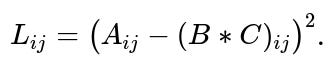
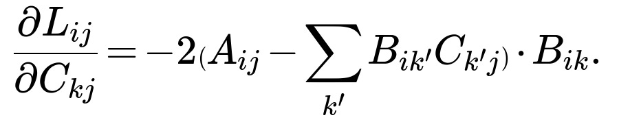
We expand (B*C)ᵢⱼ = Σₖ (Bᵢₖ Cₖⱼ). The partial derivatives are:
• For Bᵢₖ:

• For Cₖⱼ:
We then perform an update with learning rate η (a small positive constant):
• Bᵢₖ ← Bᵢₖ - η * (∂Lᵢⱼ / ∂Bᵢₖ) • Cₖⱼ ← Cₖⱼ - η * (∂Lᵢⱼ / ∂Cₖⱼ)
By cycling through many entries (or small batches of entries) of A, over many epochs, B and C get updated such that the product B*C becomes a better approximation of A.
Why This Works
This approach is essentially performing a simple two-layer linear model. If d is chosen to be smaller than either m or n, we are compressing the original matrix A into two smaller matrices, capturing underlying structures such as latent factors (e.g., in recommendation systems, these factors often correspond to hidden user/item characteristics).
Because we rely on gradient-based updates, as long as the learning rate is appropriately tuned and the data is well-conditioned, B*C converges to a factorization that minimizes the chosen loss.
Potential Implementation in Python (Using PyTorch)
Below is a simplified example demonstrating how we might implement a basic version of this using mini-batch SGD in PyTorch. Of course, this is just a conceptual illustration; in practice, you’d add data loading, GPU usage, learning rate schedules, etc.
import torch
import torch.nn as nn
import torch.optim as optim

# Suppose A is our matrix of size m x n
m, n, d = 100, 80, 20
A = torch.randn(m, n)

# Initialize B, C
B = nn.Parameter(torch.randn(m, d))
C = nn.Parameter(torch.randn(d, n))

# Define optimizer
optimizer = optim.SGD([B, C], lr=0.001)

# Loss function: MSE
loss_fn = nn.MSELoss()

# Number of epochs (illustrative)
num_epochs = 1000

for epoch in range(num_epochs):
    optimizer.zero_grad()

    # Predicted A = B*C
    A_pred = B @ C

    # Compute loss
    loss = loss_fn(A_pred, A)

    # Backprop
    loss.backward()

    # Update
    optimizer.step()

    # Optional: print progress
    if (epoch+1) % 100 == 0:
        print(f"Epoch {epoch+1}/{num_epochs}, Loss: {loss.item()}")
This code shows a straightforward approach to factorizing a matrix A into B*C by minimizing the mean squared error. We do a full-batch update for simplicity. If we wanted true SGD or mini-batch SGD, we’d sample entries of A or subsets of rows/columns.
Practical Insights and Potential Pitfalls
• Choosing d. A smaller d leads to more compression (fewer parameters) but might degrade the approximation. A larger d can achieve better approximation but with potentially higher risk of overfitting and computational cost. • Initialization. Random initialization can lead to local minima or slow convergence. Techniques like orthogonal initialization or scaled uniform initialization can sometimes speed up training. • Learning Rate. Too high leads to instability and divergence, too low leads to slow convergence. • Overfitting. If d is large and we fit A exactly (especially if A is noisy), we risk memorizing noise. Regularization is important for practical settings. One can add L2 weight decay on B and C to encourage smaller norms. • Convergence. If the rank of A is truly d, we can converge (in theory) to an exact factorization with a sufficiently flexible optimization routine and no noise. Otherwise, we get the best rank-d approximation. • Sparse Data. In scenarios like recommendation systems, A is often sparse. The typical approach is to only update Bᵢₖ and Cₖⱼ for observed entries. That is a partial matrix factorization approach.
Below, we address additional follow-up questions an interviewer might pose, with in-depth answers.
How does this factorization compare to SVD in terms of uniqueness and convergence?
In the Singular Value Decomposition (SVD), for any real matrix A of shape m×n, the SVD factorization is:

U is m×r, Σ is r×r, and V^T is r×n (where r = min(m, n) or the rank of A if we take a reduced version). SVD provides an exact factorization when rank(A) = r and yields the best low-rank approximation if we truncate the singular values.
By contrast, a generic factorization A ≈ BC with B being m×d and C being d×n does not necessarily produce an exact SVD. We typically do not constrain B and C to be orthonormal or diagonal in any portion as in the SVD. Also, the solution from the gradient-based approach may not be unique: many pairs of (B, C) can yield the same product. Unlike SVD, which is unique up to certain transformations when ignoring sign flips on singular vectors, the B and C factors in gradient-based factorization can differ by an invertible transformation M (e.g., BM and M⁻¹*C yield the same product).
For convergence, SVD has closed-form solutions via linear algebra, while the gradient-based approach is iterative and can converge to local minima (though for linear least squares, it often converges well to a global minimum, especially if the problem is convex in each factor when the other factor is fixed). The difference is that SVD is a direct decomposition, while SGD-based factorization is an iterative optimization approach that can incorporate constraints, regularization, or partial data more flexibly.
What if A is rank-deficient or has missing entries?
• Rank-Deficient A. If the rank of A is strictly less than d, then an exact factorization with BC is possible (we can find B and C such that BC = A exactly) because the effective rank is smaller than or equal to d. • Missing Entries. In many real-world applications, especially collaborative filtering (like in Netflix or Amazon recommendations), A might be partially observed. One only observes certain entries of A, and the objective is to predict the missing entries. Instead of summing over all i, j, you only sum over observed entries. SGD can handle this easily: for each observed entry (i, j), you compute the partial derivative and update Bᵢₖ, Cₖⱼ accordingly. This partial or implicit factorization approach is common in large-scale recommendation systems.
How do we regularize this factorization?
To prevent overfitting and control the size of B and C, one can include an L2 regularization term:

where ( | \cdot |_F ) denotes the Frobenius norm. This penalty encourages smaller entries in B and C, improving generalization and numerical stability. We add this regularization term to the loss function:

During SGD updates, we then include the gradients of the regularization terms. This is akin to weight decay in neural networks.
What are common convergence challenges?
Vanishing/Exploding Gradients: If entries of B or C grow too large or become too small, training becomes unstable. Proper initialization and learning-rate scheduling can mitigate this.
Local Minima: Although matrix factorization with squared error is not convex in both B and C jointly, it is convex in one factor if the other is fixed. While local minima can exist, in many practical applications the landscape is benign enough that SGD converges to a good solution.
Slow Convergence: If m and n are large, computing the full gradient is expensive. Stochastic or mini-batch methods are used to scale up. Convergence can be slow but typically works well in practice with large data.
Could we do this factorization via Autoencoders?
Yes, we can interpret matrix factorization as a linear autoencoder. Suppose we have an input vector x of length n (a row of A). We feed it into a linear encoder of size d, then a linear decoder of size n, and measure reconstruction loss. This network has weight matrices W₁ (size d×n) and W₂ (size n×d). The autoencoder reconstruction is W₂( W₁ x ). If you stack the rows of W₂( W₁ x ) for all x in the matrix, you effectively get B*C. The difference is that an autoencoder also has biases and non-linearities if we choose, but a purely linear autoencoder is mathematically similar to an SVD-based approach. With a linear autoencoder of rank d, the learned factorization is closely related to the best rank-d approximation.
Could we initialize B and C with SVD and then refine with SGD?
Yes. A practical way to speed up convergence is to use the SVD of A as an initialization. We can do a rank-d truncated SVD: pick the top d singular values and corresponding singular vectors. Then:
Set B = U sqrt(Σ)
Set C = sqrt(Σ) Vᵀ
This yields B*C ≈ A right away. Then refine B and C with additional SGD steps, possibly with constraints or specialized loss terms. This typically converges faster than a random initialization.
What if we only want nonnegative entries in B or C?
In some applications, such as certain topic models or image analysis, we might want B ≥ 0 and C ≥ 0. This is the nonnegative matrix factorization (NMF) scenario. We cannot simply use standard SGD updates if we want to strictly maintain nonnegativity, unless we project B and C onto the nonnegative orthant after each update (i.e., set negative values to zero). Alternatively, specialized NMF optimization algorithms exist (e.g., coordinate descent, multiplicative updates).
If we do want to stick with SGD, a quick hack is to store unconstrained parameters in B', C' and define:
B = exp(B'), C = exp(C')
so that B, C are guaranteed to be positive. That approach, however, changes the nature of the optimization and the interpretability of B and C, though it does enforce nonnegativity.
Additional Insights on Real-World Implementations
• GPU Acceleration. For large m and n, GPU-based matrix multiplication significantly speeds up computations. Libraries like PyTorch and TensorFlow handle the gradients and kernel-level optimizations. • Data Loading. For extremely large matrices, you typically store data in a sparse format and only sample observed entries in each mini-batch. • Convergence Criteria. We often watch the reconstruction error on a validation set. If the matrix is partially observed, we watch the error on a held-out set of entries.
Follow-Up Question: How do we handle the case where d > min(m, n)? Would that be considered overparameterized, and what are the implications?
When d > min(m, n), we have more latent factors than the dimensionality might suggest is necessary. This is an overparameterization scenario because B is m×d and C is d×n, so the total number of parameters is d(m + n), which can exceed the naive dimension of A (m×n). In principle, the model might still converge to a good solution, but there are potential issues:
• Overfitting. If you have no regularization or constraints, it becomes easier to fit any noise or irrelevant structure in A. • Redundancy. If the true rank of A is r, and you choose d > r, then there is an infinite set of solutions that can represent the same product exactly. This sometimes makes optimization less stable. • Regularization or Early Stopping. Typically, you mitigate overparameterization with strong regularization or by stopping as soon as your validation error stops improving.
Follow-Up Question: How would the update rules look if we used mini-batches of rows or columns instead of single entries?
Instead of sampling a single (i, j) entry, you might sample a block of rows or columns. For example, you can take a batch of row indices ℐ. Then you look at:
• A_batch = A[ℐ, :] (the submatrix containing only those selected rows) • B_batch = B[ℐ, :] (the corresponding rows in B)
We form a prediction:
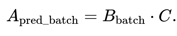
We compute a partial loss:

We then backpropagate. This updates the rows B[ℐ, :] in B and the entire matrix C. If we choose columns instead, we similarly pick columns of A and relevant columns of C. This approach can speed up training on modern hardware because matrix multiplication is more efficient than many single-entry updates.
Follow-Up Question: In practice, how large of a matrix can be factorized this way?
Modern large-scale recommendation systems factorize matrices with millions of rows and columns. However, these systems usually have only a small fraction of the total possible user-item interactions observed, so the data is extremely sparse. Advanced distributed training methods (e.g., parameter servers, sharded GPU clusters) are used to handle the computational load. The algorithm scales by sampling only observed entries (or a random subset thereof) at each step.
Follow-Up Question: How do we monitor and evaluate performance in real-world deployments?
• Reconstruction Error. On a validation set of observed entries, compute the mean squared error or mean absolute error. • Ranking Metrics. In recommendation tasks, you might measure ranking metrics (e.g., NDCG, MAP) on held-out user-item interactions. • Scalability. Monitor how the training time grows with data. Also watch memory usage. • Convergence. Track the training and validation losses across epochs or iterations.
Performance evaluation beyond simple reconstruction can include domain-specific metrics. For instance, in collaborative filtering tasks, the top-K recommendation quality is crucial.
Follow-Up Question: Could we do complex factorization objectives, such as factoring a tensor or factoring with side information?
Yes. SGD-based approaches can be generalized:
• Tensor Factorization. Instead of A being two-dimensional, we have multi-dimensional data. We can define factor matrices or factor tensors for those additional dimensions. The update rules involve partial derivatives with respect to each factor. • Side Information. Sometimes we have extra features for each row or column (e.g., user demographics or item metadata). We can incorporate them via additional terms in the model or by building a neural architecture that merges these features with the latent factors.
This flexibility is one of the main benefits of gradient-based matrix factorization: we can incorporate constraints or additional losses with relative ease.
Below are additional follow-up questions
What alternative loss functions can be used beyond MSE, and how would we implement them?
There are scenarios where the mean squared error might not be the best measure of discrepancy between A and B*C. One common alternative is the mean absolute error (MAE). Instead of squaring the residuals, MAE sums the absolute deviations. This can be more robust to outliers, because squaring large errors places a disproportionate penalty on them, whereas absolute value penalizes them linearly.
The general form of MAE for matrix factorization is
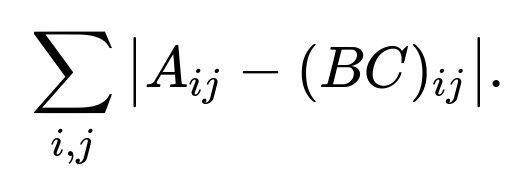
If you use MAE, you would compute gradients by differentiating the absolute value term. However, the absolute value function is not differentiable at zero, so many deep learning frameworks handle this with subgradient approximations or a smooth approximation (like the Huber loss, which transitions from L1 to L2 near zero).
In practice, you could replace the MSE loss function in your code with something like this:
import torch
import torch.nn as nn
import torch.optim as optim

def mae_loss(pred, target):
    return torch.mean(torch.abs(pred - target))

# Suppose you define B and C as before
loss_fn = mae_loss  # Instead of nn.MSELoss()
Another possibility is a Huber loss (smooth L1), which is less sensitive to outliers than MSE but differentiable at zero in a smoother way than the absolute value. This helps keep some of the benefits of MSE while limiting the impact of large errors.
Pitfalls and edge cases:
If your data has very large outliers, an L1-based loss might converge more slowly because the gradient has constant magnitude irrespective of how large the residual is.
If your matrix entries are predominantly small with only a few large spikes, you might find MSE overweighting those large spikes, making it difficult to learn smaller-scale structure. An L1 or robust loss could help.
Implementation details differ slightly among frameworks, so verifying that the subgradient or the smooth approximation is correct is important.
How can we handle memory constraints for extremely large matrices?
When m and n are very large, storing A in dense form becomes infeasible. If A is dense and truly enormous, one may need a distributed data-parallel approach. If A is sparse, you can store it in a compressed format and iterate only over the non-zero entries.
One approach to coping with memory limitations is to stream subsets of rows or columns (or even individual entries) from disk. You can sample or read these subsets, compute gradients, and discard them after updating B and C. This way, you never hold the entire matrix A in memory at once.
An additional strategy is to distribute the factorization across multiple machines. For example:
Split A into row blocks or column blocks across workers.
Each worker holds the relevant part of the matrix A and the relevant part of B or C.
Synchronize the updates for B or C that are shared across workers using a parameter server or an all-reduce operation.
Pitfalls and edge cases:
Communication overhead can dominate if not carefully controlled or if the cluster is not well provisioned for large-scale matrix ops.
If the matrix is not just large but extremely sparse, you might pay a penalty in random access patterns or overhead for indexing. Efficient sparse data structures and sampling strategies become key.
If B and C each must be distributed, you have to ensure consistent updates. Any drift or misalignment in synchronization can lead to suboptimal convergence.
What if we need an online or incremental approach where new rows (or columns) of A arrive over time?
Some real-world scenarios require continually updating the matrix factorization as new data arrives (for instance, a recommendation system in which new user ratings come in daily). In an online or incremental approach, you can keep the current estimates of B and C and update them as new rows or columns (or new entries) arrive.
For a new row i of length n (the i-th user rating vector, for example):
You initialize Bᵢ as a new row in B (often randomly or as a small constant vector).
You update Bᵢ and C by running a few steps of SGD on the observed entries in the new row.
If columns arrive, you can do the analogous procedure but for C. If both dimensions expand, the factorization must be adapted to accommodate newly added rows and columns. You might keep B and C in a data structure that can grow dynamically, or you might allocate them in large blocks upfront.
Pitfalls and edge cases:
Continual updates without careful learning rate schedules can lead to catastrophic forgetting, where updates for new data overwrite what was learned earlier.
If the newly observed data distribution differs significantly from the earlier distribution, you might need to redesign your factorization strategy or re-factor the entire matrix occasionally.
Ensuring that Bᵢ or the new columns of C converge to stable values might require mini-batch updates for the new data combined with partial re-training on old data.
Can we impose specific linear or structural constraints on B and C, and how do we do that?
Sometimes domain knowledge dictates constraints on B and C. For example, you might want Bᵢⱼ ≥ 0, or you might want certain rows to sum to one if they represent probabilities. You can incorporate these constraints in several ways.
One method is to enforce constraints via projections after each SGD step. For example, if you want nonnegativity, you clamp negative values to zero. If you need each row to sum to one, you can normalize each row by its sum. Another method is to use parameterizations that enforce constraints by construction, such as exponentiating free parameters for nonnegativity or using a softmax row-wise to ensure probability-like rows.
Pitfalls and edge cases:
Projections can disrupt gradient-based updates, sometimes causing oscillations if the learning rate is not tuned carefully.
Complex constraints (like orthogonality or block-sparsity) can require specialized optimization routines (e.g., manifold optimization).
Overly strict constraints can limit the factorization’s ability to approximate A, leading to high reconstruction error if the constraints do not align with the structure in A.
How could factorized matrices be integrated into a deep learning pipeline beyond a standalone matrix factorization?
Sometimes B*C is not the final objective but is part of a larger model. For example, in a recommendation system, the user embedding Bᵢ might be fed into a neural network that predicts user preferences, while item embedding Cⱼ might be fed into a separate network. Their dot product or a concatenation could be used as part of a more complex architecture that combines factorized embeddings with additional features.
Integration into a deep pipeline might look like this:
B and C are trainable embeddings, each row or column is an embedding vector.
The product Bᵢ · Cⱼ (or some function of these embeddings) is used along with other signals in a neural model (like user metadata, item metadata).
The entire system is trained end to end via backpropagation. The partial derivatives flow back into Bᵢ and Cⱼ.
Pitfalls and edge cases:
If the neural network is large, ensuring B and C updates do not overshadow or get overshadowed by the rest of the network updates can be tricky.
Regularizing both the embeddings and the deep model is crucial to prevent overfitting, especially if you have a small set of observed matrix entries.
Because it is a more complex model, debugging slow or incorrect convergence can be challenging if you cannot isolate the matrix factorization portion from the rest of the network.
How do we deal with extreme outliers or non-Gaussian noise distributions in A?
If A has noise that is not well-modeled by the Gaussian assumption underlying the MSE loss, you might end up chasing outliers and harming overall factorization quality. In these cases, more robust losses are preferred, such as L1 or Huber. Alternatively, you can adopt heavy-tailed distributions if you suspect your data has a Cauchy-like or Laplace-like profile, in which case you might define a negative log-likelihood with that distribution assumption.
Another strategy is to apply pre-processing or outlier detection. You can clip or down-weight extreme values in A before factorizing. This approach ensures that spurious, extremely large or small values do not dominate the factorization.
Pitfalls and edge cases:
If the outliers are actually meaningful signals (for example, a small set of extremely large values that are critical in your domain), ignoring or clipping them might cause important information to be lost.
Overly complicated robust losses can slow down optimization if not carefully implemented. Debugging subtle differences among robust loss functions is non-trivial.
How do factorized embeddings (B and C) differ from other learned embeddings in neural networks?
Matrix factorization embeddings are typically learned in a purely linear context: you have an embedding dimension d, the product of these embeddings recovers or approximates A. In a deep neural network context, embeddings are often used as initial layers, fed into one or more non-linear transformations. The matrix factorization approach is effectively a rank-d linear model, whereas deep embeddings can capture more complex relationships through non-linearity and additional layers.
Despite these conceptual differences, both approaches produce learned representations:
In matrix factorization, each row i is a latent vector in Bᵢ, and each column j is a latent vector in Cⱼ.
In a neural embedding layer, each entity (like a user or item) is assigned a learnable vector. The difference is that the subsequent network layers can reshape, combine, or transform these embeddings in non-linear ways.
Pitfalls and edge cases:
Pure factorization might converge faster because it has fewer parameters and no deep layers, but it is limited in the complexity of patterns it can capture.
Neural embeddings can overfit if the architecture is too large or not properly regularized.
Interpreting pure factorization embeddings might be simpler than deep embeddings, which can become entangled with non-linear transformations in later layers.
How do we diagnose or detect degenerate solutions in matrix factorization?
A degenerate solution is one where B or C, or both, collapse in a way that yields a misleading or trivial factorization. For instance, B might become nearly zero while C becomes extremely large (or vice versa), so that the product B*C hovers around a region that fits some portion of A but in an unstable manner.
There are a few ways to detect degeneracy:
Monitoring the norms of B and C. If you see them exploding or vanishing, you might be heading toward a degenerate solution.
Checking the reconstruction error on a validation set. If the training error plummets but the validation error remains high, it could be that the factorization is collapsing to a spurious solution or memorizing quirks in the training data.
Introducing a small regularization penalty on the norms of B and C can help push away from degenerate configurations.
Pitfalls and edge cases:
In poorly scaled data, a very large or very small step size can exacerbate degeneracy.
Some forms of degeneracy are subtle, such as solutions that appear to fit all observed entries but generalize poorly to unseen entries.
How do we incorporate domain-specific constraints like row/column sums or block structures in B and C?
In some applications, the sum of elements in each row or column of B*C might be constrained by known totals. Another scenario is block structures, where certain subsets of columns or rows must be factorized separately or share partial factors.
One approach is to add penalty terms to the loss. For instance, if you require each row sum to be close to a known value, you can define:

where Tᵢ is the known sum for row i. You then add that penalty to your main reconstruction loss.
Another approach is to explicitly encode the constraint in the parameterization of B or C (for example, using specialized layers or transformations that ensure each row or column meets the constraints).
Pitfalls and edge cases:
Hard constraints can slow down or complicate convergence if you enforce them strictly at every iteration.
Soft constraints (penalty terms) allow small violations but might never enforce exact equality, so deciding how large a penalty coefficient to use can be tricky.
Complex constraints can lead to a non-convex optimization problem with many local minima, requiring careful initialization or advanced optimization techniques.
What advanced optimizers can we use beyond standard SGD, and do they help?
While plain SGD with momentum can work, especially for smaller matrices, large-scale matrix factorization often benefits from adaptive optimizers. Examples include Adam, Adagrad, RMSProp, and others. The advantage is that these methods adjust the effective learning rate for each parameter based on the history of gradients, which can speed up convergence and reduce sensitivity to initial learning rate choices.
For matrix factorization, an adaptive optimizer like Adam might handle the varying scales of B and C entries more gracefully:
import torch
import torch.nn as nn
import torch.optim as optim

B = nn.Parameter(torch.randn(m, d))
C = nn.Parameter(torch.randn(d, n))

optimizer = optim.Adam([B, C], lr=0.01)
Pitfalls and edge cases:
Over-reliance on adaptivity can mask underlying issues with your factorization (such as poor initialization or degenerate solutions).
In large-scale distributed setups, the memory overhead for Adam’s state (which stores first- and second-moment estimates) might be high if you have tens or hundreds of millions of parameters.
Adaptive methods can sometimes overshoot or converge to suboptimal points if the learning rate is still not well tuned.
How can multiple matrices that share dimensions be factorized together with shared latent factors?
In certain multi-relational settings (for instance, user–item matrices for different categories of items), you may want to factorize multiple matrices A₁, A₂, … that each share at least one dimension (say the user dimension). This can be done by sharing the portion of the factorization for that dimension and giving each matrix its own factor for the other dimension.
For example, if you have A₁: users × items1, and A₂: users × items2, you can share the user embeddings across both A₁ and A₂ while having separate item embeddings for the two item sets. You can define your joint loss as:

where B is the shared user embedding matrix, and C₁, C₂ are item embedding matrices for the respective item spaces.
Pitfalls and edge cases:
The dimension of the latent factors must be chosen carefully to represent all tasks adequately.
If one matrix is much larger or has a different data distribution, it might dominate the updates.
There can be a trade-off between cross-task generalization (sharing user factors helps capture consistent user traits) and task-specific specialization (items in different categories might require distinct embeddings).
How can a Bayesian perspective be introduced, and what difference does it make?
A Bayesian treatment of matrix factorization treats B and C as random variables with prior distributions. A common choice is a Gaussian prior:

The likelihood of A given B and C could also be defined, for example, as a Gaussian likelihood centered at B*C. Bayesian matrix factorization then tries to infer the posterior distribution of B and C. Traditional approaches use MCMC or variational inference. In a gradient-based framework, you could perform variational inference by parameterizing distributions over B and C (like a mean and variance for each entry) and optimizing an evidence lower bound (ELBO).
Pitfalls and edge cases:
Computational overhead for Bayesian methods is typically much higher than point estimation.
Storing posterior distributions for large B and C can become infeasible unless you use factorized approximations.
Convergence can be sensitive to the choice of priors. If the priors are too restrictive, the factorization may not capture critical structure in A.
How do we handle extremely sparse data that has a large portion of unobserved or zero entries?
If the matrix is extremely sparse (for example, in recommendation systems where most users do not rate most items), storing a dense matrix is impractical. One solution is to only store the non-zero (or observed) entries in a list or coordinate format. Stochastic gradient descent can then sample from these observed entries to compute updates for B and C.
In such cases, you do not sum over all i, j in the objective but rather only over the observed entries (i, j) ∈ Ω, where Ω is the set of observed data points. If you also want to predict zeros accurately or treat them as meaningful signals, you must incorporate them explicitly into your loss. Alternatively, you might treat zeros as unobserved, which is a typical approach in user–item rating scenarios.
Pitfalls and edge cases:
If you treat zeros as unobserved, you might overpredict negative or zero-like values because the factorization might interpret the lack of data as zero. A careful choice of weighting for missing entries can help mitigate this.
When the data is extremely sparse, the updates might be slow to propagate across B and C, because only a few entries are updated at a time. Efficient sampling strategies that ensure coverage of all rows and columns are important.
If certain rows or columns have no observed entries, they become entirely unidentifiable. Handling these users or items can require additional side information or assumptions.
How do we extend matrix factorization to address a classification or multi-label scenario?
Sometimes each entry in A is not a continuous value but a label or a probability class. In that case, you might use a classification loss or a cross-entropy–based objective rather than a regression-based MSE or MAE. For instance, if each entry Aᵢⱼ is binary, you might define:

where ( \sigma(x) ) is the logistic sigmoid function. This is effectively logistic matrix factorization. The approach is similar, but you use the derivative of the cross-entropy instead of MSE. Stochastic updates then proceed by sampling entries (i, j), computing the predicted probability from Bᵢ and Cⱼ, and updating accordingly.
Pitfalls and edge cases:
Class imbalance can cause the model to become biased if one label is much more frequent than another. Weighting positive and negative examples differently might be required.
For multi-class or multi-label tasks, you need a suitable generalization of logistic or cross-entropy losses, which can be more complex to implement.
If your data is extremely sparse, you still have the same concerns about coverage and partial observability of the matrix entries.
How can we incorporate time-dependent or temporal information into the factorization?
Some data has an inherent temporal dimension, such as a user–item rating evolving over months or years. One approach is to break A into multiple snapshots (A(t₁), A(t₂), …) at different times. You can then factorize each snapshot but share or slowly evolve the factors across time. For instance, you can let B(t) or C(t) be time-varying latent factors, with a penalty for large changes between t and t+1:

This encourages smooth evolution of B and C while allowing them to adjust to new data over time.
Pitfalls and edge cases:
If data changes abruptly, forcing smooth transitions might hurt the model’s ability to adapt quickly.
If some slices (snapshots) have only partial data, the temporal model might overfit to well-covered time periods while ignoring or performing poorly on sparse intervals.
Computational complexity can multiply by the number of time slices you include, so you may need efficient incremental methods that update B(t) and C(t) only slightly from their previous state.