
ML Interview Q Series: Finding Expected Draws for Uniform Sum > 1 Using Integral & Differential Equations.
Browse all the Probability Interview Questions here.
Suppose we repeatedly sample from independent Uniform(0,1) random variables, one after another, until the sum of our samples first exceeds 1. How many draws should we expect to make?
Short Compact solution
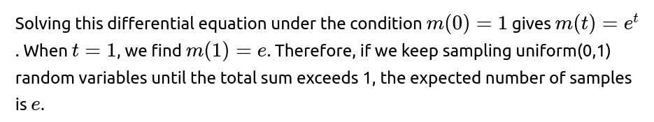
Define a function m(t) as the expected number of samples needed so that the partial sum of i.i.d. Uniform(0,1) draws first exceeds a threshold t. If the very first draw x is greater than t, then we only needed 1 draw. Otherwise, if x<t, then we already used 1 draw, and we still need however many draws are expected to exceed (t−x). Hence

A change of variables u=t−x turns the integral into an integral in u from 0 to t. This leads to
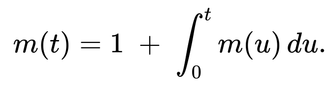
Differentiating both sides with respect to t yields

Comprehensive Explanation
To see why the expected value comes out to e, it can help to think about how the problem involves a “stopping time” setup, where we stop sampling exactly when the total goes above 1. The essence of the integral equation is that each sample is uniform on (0,1) and, given a threshold t, either the first sample alone pushes us over t or it partially “uses up” some amount less than t, leaving t−x to go. This naturally produces the relation:
When the first sample x is at least t, no further samples are needed. Otherwise, you pay 1 sample plus whatever the expected cost is for the reduced problem with a smaller threshold t−x. The uniform distribution means we integrate m(t−x) over x from 0 to t. Solving that integral equation is a standard differential-equation exercise and reveals the exponential form.

Because e is around 2.71828, it indicates that on average you need roughly three draws (on occasion you’ll need fewer, and sometimes more, but across many simulations you’ll end up with an overall average close to e).
A practical way to build intuition is to code a short simulation and observe that, over many trials, the average number of samples needed approaches e.
Potential Follow Up Question: Could we verify this result through a simple simulation?
Yes. For instance, you could write a quick Python script to repeatedly generate Uniform(0,1) samples until the sum exceeds 1, track how many draws were needed, and then average the total draws across all trials.
import random
import statistics

def expected_num_draws(trials=10_000_00):
    counts = []
    for _ in range(trials):
        s = 0
        count = 0
        while s <= 1:
            s += random.random()
            count += 1
        counts.append(count)
    return statistics.mean(counts)

print(expected_num_draws())
As you increase the number of trials, the printed mean should get closer and closer to e≈2.71828.
Potential Follow Up Question: Why does the integral equation turn into a differential equation?
The core functional equation is


Potential Follow Up Question: How does this result generalize to other distributions besides Uniform(0,1)?
If the distribution is not uniform, say an exponential distribution with mean 1, or some other continuous distribution, you can still set up a similar recursive or integral-based argument. However, the shape of the integral equation would be different because the probability that a single draw surpasses t is tied to the distribution’s cumulative distribution function. For instance, if you were using exponential(1) random variables, you would find a different form for m(t). Each distribution leads to a different functional equation, and the expectation of the stopping time can differ significantly from e in those cases. The uniform distribution’s simplicity is what yields the neat exponential solution.
All these considerations show that while the problem is elegantly solved using the differential equation for Uniform(0,1), in real interview or research settings it’s important to be able to adapt the reasoning to other distributions or more complex constraints.
Below are additional follow-up questions
If the random variables were discrete instead of continuous, how would the analysis change?
When we shift from continuous Uniform(0,1) random variables to discrete variables, the integral equation approach transforms into a summation-based recurrence. Instead of forming an integral for the expectation, we would form a discrete recursion.

If x>t, then we exceed t in one draw. Otherwise, if x≤t, we pay 1 draw plus whatever is expected to exceed t−x. Symbolically, for integer-valued X, you would have something like:

This equation can often be rearranged and simplified to a more direct form. However, it may require careful bounding if the state space is large or infinite. The difference is that we no longer get a neat differential equation. Instead, we get a difference equation or discrete recursion. Solving such a recursion often involves identifying patterns, generating functions, or other combinatorial techniques.
A typical pitfall is forgetting that in discrete settings, your first draw might jump well past the threshold or only partially toward it. Failing to account for probabilities of different discrete values can give an incorrect expectation formula.
What happens if we require the sum to exceed 1 by at least a certain margin, say 1 + δ?
Now we want to stop as soon as our partial sum exceeds 1+δ, where δ>0. The primary conceptual difference is that the threshold we need to surpass is higher than 1. From a purely mathematical standpoint, we can define m(t) for all t≥0 in the same way: the expected number of draws needed for a sum of Uniform(0,1) to exceed t. Then we specifically want m(1+δ).
The same integral equation approach works:


One real-world subtlety is that as you raise the threshold beyond 1, it becomes ever more likely you need multiple draws. That will in turn affect the shape of the solution. It is a bit more involved than the t=1 case, but the process is the same.
How would correlated samples instead of independent Uniform(0,1) variables affect the approach?
Once you introduce correlations, the standard short integral/differential equation method breaks down because the expectation of the stopping time can no longer be decomposed purely based on the remainder t−x. The independence assumption was crucial in deriving

If samples are correlated, the distribution of the next sample given the previous sums is no longer simply the uniform distribution on (0,1). Hence, the transition from t to t−x is no longer uniform, so you can’t do a straightforward integral over that domain with a constant density.
One potential pitfall is to try to use the same integral approach without considering correlation. That would produce an incorrect formula for m(t). In correlated scenarios, you’d have to define m(s,n) as the expected additional draws needed given that the current sum is s and some knowledge about the distribution of the next draw that depends on past draws. You might end up with a more complex Markov chain or a non-Markovian process depending on the structure of the correlation. Analytical solutions often become much more challenging, so numerical or simulation-based approaches might be more practical.
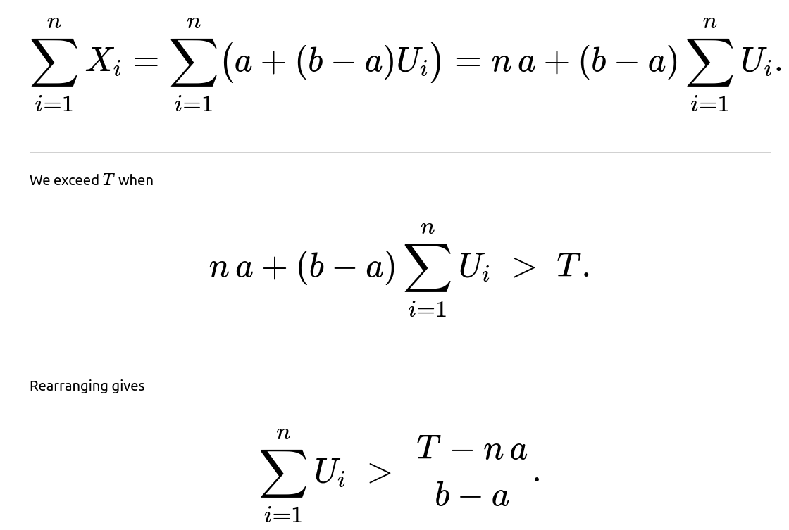
Can we adapt the methodology if the draws are not on (0,1) but on (a,b)?
When you move to a Uniform(a,b) distribution, you can shift and scale the problem. A Uniform(a,b) random variable X can be converted to a Uniform(0,1) random variable by the transformation:


What if we have only a limited budget of draws, say a maximum of N draws, to exceed 1?
In this constrained version, we can’t draw indefinitely. We have at most N trials to surpass 1. Here, we might be interested in two related questions:
The probability that we successfully exceed 1 within N draws.
The expected number of draws used, given that we always stop either when we exceed 1 or when we run out of draws (whichever happens first).
For the probability-based question, a geometric or volume-based approach can still be used. Specifically, the event that we do not exceed 1 after n draws is the same as all partial sums being at most 1, implying:
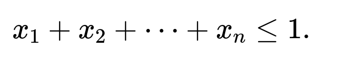
For Uniform(0,1) variables, that region in n-dimensional space is the standard simplex, whose volume is 1/n!. So the probability that n draws remain below 1 is 1/n!. If you have a limited budget of N draws, you can compute the probability of failing to exceed 1 with up to N draws by looking at that region’s volume. Then you can sum up the probabilities of not exceeding 1 after 1,2,…,N draws. The details vary depending on whether you want the distribution of the stopping time or just a final success/failure probability.
For the expected stopping time with a cap of N draws, you have:
With probability that you exceed 1 in fewer than N draws, your stopping time is the random variable from the original problem (truncated).
With probability that you never exceed 1 in those N draws, your stopping time is N.
A pitfall is to simply assume the expected stopping time remains e. Actually, e is only valid if we can go on indefinitely. If N is relatively small, then we are artificially forced to stop if we haven’t exceeded 1 by the N-th draw, and that changes the distribution of the stopping time. In the limit as N goes to infinity, we recover the original result that the expectation is e.
What if our threshold itself is random rather than fixed at 1?
If the threshold is a random variable, say T, you would be looking at E[N] where N depends on a random threshold T and i.i.d. Uniform(0,1) draws. Then you have to condition on T:

The subtlety arises if T can take values beyond 1 or below 0. You must handle each scenario appropriately: for t≤0, you might instantly exceed t with 0 or 1 draws, whereas for t>1, you have the extended threshold scenario. Another subtlety is that if T is random with a distribution that includes large values, you might need many draws quite often, and the average might be higher than e. This can sometimes drastically increase the final expectation.
How does the result generalize if we apply a “stopping rule” other than “stop the moment the sum exceeds 1”?
A stopping rule is any strategy that determines when to stop sampling based on observed values. If the rule is specifically “stop as soon as the partial sum first exceeds 1,” that is a deterministic threshold-based rule. But one might consider alternative rules, such as stopping if the sum is above 1 or if the variance of the samples so far is below some threshold, or if we suspect from partial sums that continuing isn’t worthwhile.
Analyzing these more general stopping rules typically involves martingale theory, Markov decision processes, or dynamic programming. One might define a value function that captures the expected cost or reward of continuing to sample. Then you would optimize or solve that function to find the best stopping rule.
A hidden pitfall with more complex stopping criteria is ignoring that the draws remain i.i.d. only if we keep sampling the same distribution. If any adaptive changes occur (e.g., changing the distribution of the next draw based on what we’ve seen so far), that breaks the original i.i.d. assumption and complicates the mathematics. Thus, for advanced stopping rules, you need to carefully track how your distribution or cost function changes with each draw.
What changes if, instead of summing the samples, we track their product until it exceeds 1?
Tracking the product of Uniform(0,1) random variables introduces a fundamentally different problem because you typically can’t exceed 1 by multiplying values that are each in the interval (0,1). The product tends to get smaller with each factor (unless you allow values >1, which is impossible for Uniform(0,1)). So in the product case, you might only ask: “How many draws does it take for the product to fall below some small threshold ϵ?” That is the “coupon collector of products” or a “geometric-type” question, and the expected time to cross such a boundary can be very different.
A straightforward pitfall is to think the same integral or summation approach we used for sums will apply to products. The dynamic for products is multiplicative, not additive, so you would have a recursion more akin to:
E[# steps to go below ε] = 1 + ∫ E[# steps to go below (ε / x)] f_X(x) dx
where X is the random draw. Even the boundary conditions differ, because if x<ϵ, you are already below ϵ. This demonstrates that each operation—sum vs. product—leads to an entirely different problem structure and solution approach.
If we wanted to approximate e in a real-world setting with potential floating-point inaccuracies, what numeric or rounding issues might appear?
In real-world computational environments, floating-point imprecision can affect repeated summations. If the sum of the Uniform(0,1) samples is maintained in a floating-point variable, small increments might not be accurately captured once the partial sum becomes large relative to the magnitude of each sample. However, since our threshold is only 1, this risk is somewhat small—double precision floating point can handle sums near 1 with sub–machine-epsilon increments for typical ranges.
On the other hand, if you were summing a large number of tiny increments or your threshold was extremely large, floating-point rounding could cause the sum to skip over the threshold in a single jump. You might incorrectly record fewer draws than expected or incorrectly fail to detect the exact moment the sum surpasses 1.
One common pitfall is doing naive comparisons like “if (sum > 1.0)” inside a loop without considering that sum might jump directly from 0.99999994 to 1.00000012 and skip some increments in between. Typically, to mitigate these problems, you would rely on higher-precision data types (like decimal in Python, or long double in C++ for partial improvement) or carefully arrange the order of summation.
In practice, with a moderate number of draws (the expectation is under 3, on average), floating-point inaccuracies are not usually catastrophic. Still, it’s important to be aware that in extended or more sensitive thresholds, you might need special care in summation and comparison to ensure correct results.