ML Interview Q Series: Finding Independence for Linear Combinations of Bivariate Normals via Zero Covariance.

Browse all the Probability Interview Questions here.

6. Suppose we have two random variables, X and Y, which are bivariate normal. The correlation between them is -0.2. Let A = cX + Y and B = X + cY. For what values of c are A and B independent?

Detailed Explanation of the Core Concept and Reasoning

When X and Y are jointly (bivariate) normal, any linear combinations of X and Y will also be normally distributed. For two normally distributed random variables to be independent, it is necessary and sufficient that their correlation be zero. Hence, to find for which values of c the random variables A = cX + Y and B = X + cY are independent, we look for c such that

Below is the derivation of Cov(A, B) under the assumption that X and Y have mean zero (which simplifies the correlation and covariance expressions without any loss of generality). Once we find the condition Cov(A, B) = 0, we solve for c. Because we are told the correlation between X and Y is -0.2, we can either use the general variance and covariance symbols or make the simplifying assumption of unit variances. In many interview contexts, it is standard to assume X and Y each have variance 1 unless specified otherwise. The bivariate normal correlation of -0.2 implies

Under that standard normal assumption, we have:

A = cX + Y B = X + cY

We compute Cov(A, B) as follows:

Since covariance is bilinear,

When X and Y have variance 1 and correlation -0.2, we get:

Substituting these values in:

Combine like terms:

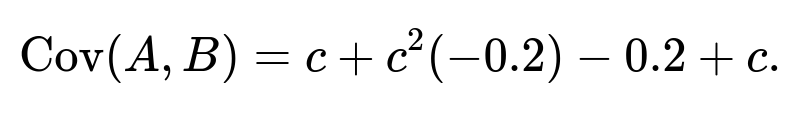
Rewrite it more neatly:

We want this to be zero:

Multiplying both sides by -5 for clarity:

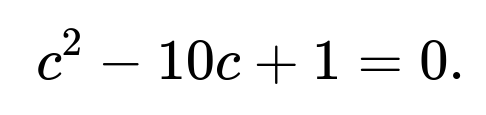
This is a standard quadratic equation in c. The solutions are given by the quadratic formula:

Thus, for X and Y bivariate normal with correlation -0.2 and unit variances, the two values of c that make A and B independent are

Setting that expression to zero yields a quadratic equation in c. Solving that equation will yield a similar form. However, in many interview questions (and especially with the numeric correlation -0.2 provided), it is common to assume X and Y have unit variance unless otherwise specified, hence the simpler numeric final result above.

The fundamental idea is: for any two random variables that are linear combinations of jointly Gaussian variables, zero covariance implies independence. This crucial fact holds only because X and Y are jointly normal. If X and Y were not jointly normal, zero covariance (or zero correlation) would not guarantee independence.

How We Know Setting Cov(A, B) = 0 Ensures Independence Here

In a bivariate normal setting, (A, B) also form a jointly normal pair. For jointly normal pairs, the condition Corr(A, B) = 0 is equivalent to independence. This does not generally hold in non-normal distributions.

Possible Subtle Points

It is worth noting a few real-world considerations or subtleties that might come up in deeper discussions:

If the correlation between X and Y was different (e.g., 0.5 or -0.8), or if their variances were not both equal to 1, the resulting values of c would differ. The main takeaway is that the independence condition is always determined by forcing the covariance between A and B to zero when (A, B) are jointly normal.

If X and Y had non-zero means, we could shift them to zero mean by subtracting their means (i.e., define

). Since linear shifts do not affect covariance or correlation, the condition for independence (in terms of c) would remain the same.

A potential interview pitfall is to assume that zero correlation always implies independence in general. This is only guaranteed for the special case where the pair is jointly Gaussian (or in certain other specialized distributions). Otherwise, uncorrelated variables might still be dependent. The difference between uncorrelatedness and independence is a standard conceptual check in interviews.

Follow-up Question 1

If we did not assume that X and Y have unit variances, how would the result change?

In that more general case, assume

Define again:

A = cX + Y B = X + cY

Then the covariance is:

Set it to zero to find c:

This is a quadratic in c:

Solving via the quadratic formula:

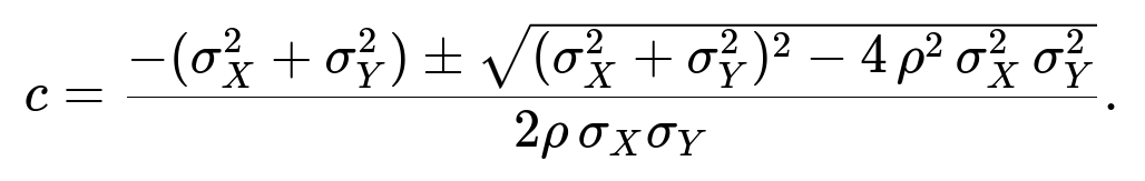
Hence, for the general variances

, you would get two possible real values of c (assuming the expression under the square root is nonnegative). In an interview, you might simply provide either the final formula or note that in the special case

Follow-up Question 2

Why can we rely on Cov(A, B) = 0 to guarantee independence for this particular problem?

For a pair of random variables to be independent given that they are jointly normal, it suffices (and is necessary) that their correlation be zero. Any linear combination of two jointly normal variables results in another jointly normal pair. Hence, if (X, Y) are bivariate normal, then (A, B) defined by linear transformations of X and Y are also jointly normal. In a jointly normal setting, zero correlation always implies independence.

However, if X and Y were not jointly normal, zero correlation between A and B would not necessarily imply that A and B are independent.

Follow-up Question 3

Could there be any numerical or edge-case pitfalls?

One potential edge case arises if

(i.e., X and Y are uncorrelated to begin with, or one has zero variance). Then the quadratic formula might degenerate or yield strange values (e.g., dividing by zero). Another pitfall is if the expression under the square root becomes negative, indicating no real values of c exist that make Cov(A, B) = 0. This would occur if

which means you cannot find a real c in that scenario. For typical correlation magnitudes less than 1 and positive variances, though, you will usually find two real solutions.

A further subtlety can occur if in practice you do not have perfect knowledge of the correlation (for instance, it might be estimated from data). Then the real-world solution for c might be approximate, reflecting the uncertainty in your estimate of

Follow-up Question 4

What happens if we accidentally rely on zero correlation for non-normal variables?

Zero correlation alone does not imply independence for arbitrary distributions. For example, in certain cases (like a symmetric distribution of X and Y around zero but with a nonlinear dependence), X and Y can have zero correlation yet remain dependent. The key reason it works here is the assumption of joint normality. Interviewers often want to see if the candidate can make that distinction: correlation being zero is not generally enough for independence, unless we have the normality assumption or some other special structure.

Follow-up Question 5

Could you provide a short Python example illustrating how one might check independence numerically?

Below is a simple snippet in Python. We generate X and Y with correlation -0.2 and assume each has variance 1. We then form A and B for the two computed values of c. Finally, we check if the empirical correlation of A and B is close to zero:

import numpy as np

np.random.seed(42)

# Number of samples
n = 10_000_000

# Correlation
rho = -0.2

# Generate X, Y as standard normal with correlation rho
# We can use Cholesky of covariance matrix or direct methods
mean = [0, 0]
cov = [[1, rho],
       [rho, 1]]

X, Y = np.random.multivariate_normal(mean, cov, size=n).T

# Compute the two possible c values:
# From the derived quadratic c^2 - 10c + 1 = 0 => c = 5 ± 2 sqrt(6)
c1 = 5 + 2*np.sqrt(6)
c2 = 5 - 2*np.sqrt(6)

# For each c, define A = cX + Y, B = X + cY
for c in [c1, c2]:
    A = c*X + Y
    B = X + c*Y
    corr_AB = np.corrcoef(A, B)[0, 1]
    print(f"c = {c}, Empirical corr(A, B) = {corr_AB:.6f}")

This example (with a large n) would yield empirical correlations near zero for the two values of c that we derived, confirming that they are effectively uncorrelated in practice for a large sample, and thus close to being independent when the data truly follows a bivariate normal distribution with correlation -0.2.

In a real-world scenario, you might not know

ρ

or the variances exactly, but the principle remains: for bivariate normal data, the values of c that force Cov(A, B) = 0 are precisely those that make A and B independent.

---

Below are additional follow-up questions

How does this analysis extend if we consider a trivariate or higher-dimensional normal scenario with more correlated variables?

When we move beyond two variables and consider a higher-dimensional normal distribution, the fundamental principle that zero covariance implies independence still holds, but only if the entire vector of random variables is jointly Gaussian. In a trivariate or higher-dimensional normal setting, linear combinations remain jointly Gaussian. However, one subtlety is that independence between two specific linear combinations in a higher-dimensional setting may depend on the correlations (and covariances) those linear combinations have with all other variables in the set, not just the pair under immediate consideration.

It can sometimes happen that the constraints required to make two combinations uncorrelated in a higher-dimensional space become more intricate. For instance, in a trivariate normal distribution with variables X, Y, and Z, if you define two linear combinations involving all three variables, you would need to solve a system of equations to ensure their mutual covariance is zero. A key pitfall arises if you assume that forcing certain pairwise covariances to zero is sufficient for independence without verifying that no other dependencies remain in the broader joint structure. Because independence in a jointly normal system can be considered by looking at the covariance matrix as a whole, one must systematically ensure that the off-diagonal blocks of the covariance matrix vanish between the relevant combinations.

In real-world scenarios, data might not perfectly follow a multivariate normal distribution, which complicates the independence argument. Zero covariance in higher dimensions does not necessarily imply independence unless you have established or can approximate joint normality. Additionally, practical constraints, such as not having enough samples to reliably estimate the full covariance matrix, can affect how accurately you identify those linear combinations that might be uncorrelated or independent in a high-dimensional setting.

What happens if we only have sample estimates of the correlation and covariance, and we attempt to solve for c based on those estimates?

In practical machine learning or statistical analysis, we rarely know the exact values of correlations and variances. Instead, we have sample estimates from data. If we attempt to solve for c by replacing the true parameters (like the true correlation

ρ

or the true variances

) with sample estimates, we get an estimate of c rather than an exact value.

This estimation introduces uncertainty because sample correlations and variances are themselves random variables subject to sampling error, especially if the dataset is not sufficiently large. The estimated c might vary significantly depending on the sample used, leading to possible overfitting if we rely on these parameters too strongly in a model-building context.

In real-world applications, one might construct confidence intervals for c. For example, you can bootstrap your sample multiple times to get a distribution of the estimated correlation and variance values, then solve for c in each bootstrap replicate. This would give you an empirical distribution of possible c values. A key pitfall here is that if your sample size is small or if the true correlation is close to zero, the estimation variance for

ρ

might be large, which can produce a wide range of c estimates. Moreover, in real datasets that deviate from normality, the sampling distributions of correlation estimators can be skewed, further complicating the inference process.

How would we interpret the scenario if correlation is exactly -1 or +1, given the formulas we derived?

If X and Y are perfectly correlated (correlation of +1 or -1), they are linearly dependent, meaning one can be expressed exactly as a scalar multiple of the other. For instance, if

ρ=+1

, we essentially have Y = aX for some a with probability 1 (assuming non-zero variances). If

ρ=−1

, Y = -bX for some b. In either case, you lose the degrees of freedom to form interesting combinations that are independent because, effectively, there is just a single unique underlying random variable driving both X and Y.

In the formula for Cov(A, B) to be zero, you could end up with degenerate conditions or potential divisions by zero when you incorporate perfect correlations. If

ρ=+1

or

ρ=−1

, the determinant of the covariance matrix for (X, Y) is zero, which signals perfect collinearity. Substituting those values into the quadratic expressions we had can cause the discriminant to vanish or become undefined, meaning no real solution for c that yields independence other than contrived cases where A or B collapse to a constant zero random variable. In other words, if X and Y are perfectly correlated or anti-correlated, A and B cannot be independent unless one of them is identically zero or they are the same up to a sign factor.

In practical terms, perfect correlation is rarely observed in real data, but near-perfect correlation can still cause numerical instability in computations (e.g., near-singular covariance matrices). This can be a pitfall in machine learning pipelines, especially if you rely on matrix inversions or gradient-based methods where near-singularities can lead to exploding parameters or indefinite Hessians.

Could there be situations in which nonlinearity or transformations of X and Y affect the independence of A and B?

When X and Y are bivariate normal, any linear combination stays in the same linear domain, and independence of these linear combinations hinges on zero covariance. However, if we apply nonlinear transformations—for example, A =

cX+Y

but B =

, or B = log

(X+cY)

—then even in the bivariate normal setting, we no longer have a straightforward guarantee that zero covariance of transformed variables leads to independence.

The reason is that bivariate normal distribution properties are preserved under linear transformations, not under arbitrary nonlinear transformations. A subtlety emerges if you transform X or Y to X' = g(X) and Y' = h(Y) for some nonlinear g, h. Then, even if X and Y were originally normal, (X', Y') may not have a joint distribution that remains “nice,” and the independence arguments using only linear covariance can fail.

In a real-world scenario, transformations are often used to stabilize variance or to induce approximate normality (like Box-Cox transformations). One must carefully check whether these transformations preserve or destroy the linear correlation structure. A pitfall is to assume that independence is implied by zero correlation after transformations. This assumption typically requires verifying that the transformed pair is still jointly normal or at least verifying independence through more direct means (e.g., performing tests for mutual information).

Are there practical applications where one might deliberately construct such linear combinations to achieve independence?

One practical application is in constructing portfolios in finance. If X and Y represent returns on two different assets and you want to combine them into a new pair of portfolios that are as uncorrelated (or independent) as possible, you might adjust the weights (analogous to c) to achieve minimal covariance between them. Although independence is a strong condition (and real market returns rarely obey strict normality), the principle of seeking uncorrelated portfolios is quite common.

Another example appears in signal processing, where you might want to separate signals (e.g., for blind source separation) using techniques like Independent Component Analysis (ICA). While ICA often relies on higher-order statistics beyond covariance, certain simpler algorithms might start by enforcing zero correlation in linear mixtures as a first step. A subtlety is that zero correlation is just one constraint, and achieving full independence might require additional constraints or transformations (since many real-world signals do not follow normal distributions).

A pitfall arises when applying these methods blindly: you might only reduce correlation at the second-order (i.e., covariance) level without truly achieving independence in higher-order moments. This is especially relevant if you rely on the assumption of normality, which can be incorrect for non-Gaussian signals or data series.

What if the random variables X and Y have unequal sample sizes or come from slightly different distributions?

Sometimes in practice, you might have data for X from one source or time period and data for Y from another source or partially overlapping time intervals. If you try to combine them in the manner A = cX + Y and B = X + cY, you have to handle missing data or mismatched sample sizes. One approach is to only analyze the time (or index) range where both X and Y are simultaneously observed, effectively discarding extra data from either side. This can reduce your effective sample size, thus increasing variance in the covariance estimates.

Additionally, if the distributions of X and Y are not precisely normal—say Y has a heavier tail or a different shape—then the theoretical property that zero covariance implies independence no longer holds strictly. You might use transformations or robust estimation techniques (like rank-based correlation measures) to get a better sense of the dependence structure. A potential pitfall is to proceed with the normal-theory formulas and interpret the results as if they guaranteed independence, when, in fact, you are only capturing linear relationships with respect to the overlapping segments of data.

How do outliers or heavy tails impact the numerical stability of solving Cov(A, B) = 0?

In real data, especially from domains such as finance, e-commerce, or user activity logs, heavy-tailed distributions are common. Outliers can greatly affect sample covariance estimates. Because covariance is sensitive to extreme values, a few large outliers in X or Y can skew the estimated correlation or variances, leading to an inaccurately computed c if you rely on those sample estimates.

Heavy tails can also make confidence intervals around correlation or variance estimates much wider, so the numeric solution for c might not be reliable. Practically, if the data exhibit outliers, you might consider robust methods for covariance estimation (e.g., M-estimators or minimum covariance determinant estimators). A pitfall is ignoring the presence of outliers, which can produce a spurious solution for c that does not generalize. This is particularly critical in any domain where extremes can occur with non-trivial probability, such as risk assessment or anomaly detection.

What modifications are necessary if we want to force A and B to be orthogonal in a least-squares sense (rather than merely uncorrelated)?

If you interpret A and B as vectors in a high-dimensional feature space (e.g., each sample of A and B seen as coordinates in a long vector), being orthogonal in the Euclidean sense can differ from being uncorrelated as random variables. Orthogonality in a least-squares or geometry sense might require you to consider dot products of sample vectors after some transformation or standardization.

Although in probability theory, “uncorrelatedness” is often called orthogonality in L2 space, in a machine learning context with sample-based data, one might define orthogonality differently. For instance, you may want the empirical average of A times B to be zero, which is akin to sample-based uncorrelatedness. A subtlety is that if you only impose orthogonality on the sample vectors for a particular batch or data segment, you might not guarantee true independence. The pitfall is failing to distinguish between these different notions of orthogonality and inadvertently concluding independence from a purely geometric constraint. In essence, random variable independence is a stronger condition than being uncorrelated over a finite sample or being orthogonal in a Euclidean sense for one batch of data.

How might knowledge of independence between A and B help in a machine learning feature engineering context?

In feature engineering, one common practice is to transform or combine existing features to reduce redundancy. If A and B are truly independent, each might capture distinct information about the target variable in a regression or classification task. This can reduce multicollinearity, leading to more stable parameter estimates in linear models and potentially improving generalization for certain algorithms.

However, a major subtlety is that independence among features does not necessarily guarantee better predictive performance unless that independence also aligns with the target variable’s predictive structure. Another pitfall is ignoring interactions with the label: two features can be marginally independent yet jointly correlated with the label in a complex nonlinear manner. For example, each feature might be uninformative alone, but together they provide strong predictive signals. So, while seeking uncorrelated or independent features is conceptually appealing for simpler models (like linear regression), advanced models (random forests, gradient boosting, deep networks) can automatically discover intricate dependencies between features.

Can we extend this concept to partial independence, where we condition on a third variable?

Partial independence refers to the notion that two random variables A and B might be independent given a third variable Z. In classical statistics, this is captured by conditional independence statements, often checked via partial correlations in a multivariate normal setting. If X and Y are bivariate normal, and we define A and B as linear combinations of X and Y plus potentially some third variable Z, we may want to check if Cov(A, B | Z) = 0 as a condition for conditional independence.

In a practical situation with conditioning, you need to look at the conditional covariance matrix. For instance, in a three-variable normal system X, Y, Z, the partial correlation between X and Y given Z is computed from the inverse of the covariance matrix (the precision matrix). If you try to ensure independence of A and B conditional on Z, you might solve a more complex system involving partial correlations, not just the raw pairwise correlations. A pitfall here is ignoring the partial correlation concept and incorrectly concluding independence when you have not accounted for a third or additional variables that might create spurious correlations or block paths of dependence.