ML Interview Q Series: Finding Lines and Hyperplanes in High Dimensions Using PCA/SVD

📚 Browse the full ML Interview series here.

11. Suppose I have (10000, 100) data points with 100 dimensions, all of them lying on a hyperplane. What is the equation of the line?

Understanding the question requires untangling two key concepts: the idea of a “line” in a high-dimensional space versus a “hyperplane.” In a 100-dimensional space:

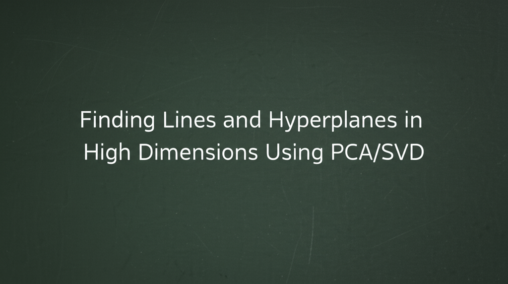
A hyperplane is a 99-dimensional affine subspace. Its standard linear equation can be written as

where (x) is any point (a vector in (\mathbb{R}^{100})), (w \in \mathbb{R}^{100}) is the (non-zero) normal vector to the hyperplane, and (b) is a scalar offset.

A line is a 1-dimensional subspace (plus a shift if not through the origin). Its equation is often written in parametric form. If the data truly lie on a single line in (\mathbb{R}^{100}), you can represent that line as

x(t)=a+tv

where (a \in \mathbb{R}^{100}) is a point on the line and (v \in \mathbb{R}^{100}) is the direction vector.

In many geometry or machine-learning contexts, one might say “the data all lie on a hyperplane,” but if it is strictly a hyperplane, then that subspace has dimension 99 (not dimension 1). If, instead, they actually all lie on a line (dimension 1), that line is a much smaller subspace. Sometimes, the term “hyperplane” is used loosely for any lower-dimensional affine subspace in a high-dimensional ambient space, though that can be imprecise.

Below is a detailed discussion of how one would find the equation of a line in (\mathbb{R}^{100}) if the data are collinear (truly lie on a 1D subspace) and how one would find the equation of a hyperplane if they lie on a 99D subspace.

Finding the line if the points are truly collinear

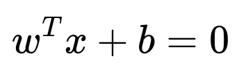
Identify two distinct points from the 10,000 data points, call them (x^{(1)}) and (x^{(2)}). These points must be different vectors in (\mathbb{R}^{100}). Form the direction vector

Choose (a = x^{(1)}) as a reference point on the line. Then any point (x) on this line can be written in parametric form as

x(t)=a+tv.

Here, (t) is a scalar parameter. If the data truly lie on this line, then every data point (x^{(i)}) will satisfy that equation for some value of (t).

Finding the hyperplane if the points lie on a 99-dimensional affine subspace

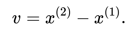
A hyperplane in (\mathbb{R}^{100}) can be described by a single linear equation of the form

where (w \in \mathbb{R}^{100}) and (b \in \mathbb{R}). To find (w) and (b), you need to determine the normal vector that is orthogonal to that 99-dimensional subspace. For instance, if your data truly spans 99 dimensions, you can compute the singular value decomposition (SVD) or principal component analysis (PCA). The smallest singular value (or the last principal component) might reveal the direction perpendicular to the hyperplane. That direction becomes (w), and you can solve for (b) using the condition (w^T x^{(i)} + b = 0) for any point (x^{(i)}) on the hyperplane.

Because the question specifically says “all of them lying on a hyperplane” but then asks for “the equation of the line,” it can be a trick question. Typically, “hyperplane” in (\mathbb{R}^{100}) means dimension 99, whereas “line” means dimension 1. In interview settings, clarifying whether the subspace is truly 1D or 99D is important. The forms above show how to write down an explicit equation in each case.

Using code to illustrate how to find a line from data (if truly collinear)

import numpy as np

# Suppose data is in a NumPy array 'X' of shape (10000, 100)

# Step 1: pick two distinct points
x1 = X[0]          # shape (100,)
# Find another point distinct from x1
for i in range(1, X.shape[0]):
    if not np.allclose(X[i], x1):
        x2 = X[i]
        break

# Step 2: direction vector
v = x2 - x1

# Step 3: parametric form
# A function that gives a point on the line for parameter t
def line_point(t):
    return x1 + t * v

# line_point(t) now gives the parametric coordinates of the line

One could verify that every row of (X) (every data point) fits on this line by finding a corresponding (t). If the data are not collinear, that means they might instead lie on a higher-dimensional subspace (e.g., a hyperplane of dimension 99), in which case you switch to the normal vector approach or an SVD/PCA approach.

Subtleties and edge cases

If all 10,000 points are identical, the line (or hyperplane) is degenerate because there is no distinct direction. If the points nearly lie on a line but are not exactly collinear, numerical issues can affect whether you get an exact direction vector or a least-squares best fit line. If the question truly intended a 99D hyperplane, then only a single linear equation is needed in (\mathbb{R}^{100}). But that is not typically called “the equation of the line” because a 99D hyperplane is not a line.

Below are potential tricky interview-style follow-ups about this scenario.

How do you determine if the data truly lies on a line or a 99D hyperplane?

You can check the rank of the matrix formed by subtracting one point from all the others. If the rank is 1, the data is collinear. If the rank is at most 99, the data might lie in a 99D subspace (a hyperplane) or lower. In practice, you can use PCA:

1. Subtract the mean from all points.

2. Perform an eigendecomposition of the covariance matrix.

3. Check how many principal components have non-negligible variance. If exactly one principal component has non-zero variance, the data is collinear (a line). If exactly 99 have non-zero variance, the data lies on a hyperplane of dimension 99, and so on.

How do you handle floating-point error when checking collinearity?

In practical scenarios, you never expect data to be perfectly on a line due to floating-point or measurement noise. You typically set a tolerance. For example, you might look at the ratio of the smallest singular value to the largest singular value. If that ratio is below a threshold (like 1e-12), you can consider the data to be effectively lying in a lower-dimensional subspace. You might do:

import numpy as np

X_mean = X.mean(axis=0)
X_centered = X - X_mean
U, S, Vt = np.linalg.svd(X_centered, full_matrices=False)

# Check S from largest to smallest
if S[-1] < 1e-12:
    print("Data might be on a lower-dimensional subspace.")

Is there a direct formula for the normal vector of a hyperplane given many points?

If points ({x^{(1)}, x^{(2)}, \dots, x^{(N)}}) lie in a hyperplane, then any vector normal to that hyperplane is orthogonal to all pairwise differences (x^{(i)} - x^{(j)}). So you want a non-zero (w) that satisfies

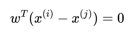
for all (i,j). Equivalently,

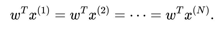
When the subspace dimension is large (99 for a hyperplane in 100D), you usually do an SVD or PCA for numerical stability. The vector (w) associated with the smallest singular value (or the last principal component) is the hyperplane’s normal.

How would you do this in code for a hyperplane?

One approach:

import numpy as np

# X is the data matrix of shape (10000, 100)

# Subtract the mean to get an affine subspace through origin
X_mean = np.mean(X, axis=0)
X_centered = X - X_mean

# SVD
U, S, Vt = np.linalg.svd(X_centered, full_matrices=False)
# The last right singular vector Vt[-1] is orthonormal to the subspace
w = Vt[-1]  # normal vector

# Then b can be computed so that w^T x + b = 0 holds for all x in X
# For the hyperplane to contain the original points:
#   w^T (x^{(i)}) + b = 0
# We can use any data point x^{(i)} to solve for b.

b = -np.dot(w, X[0])

Thus the hyperplane equation is

This method is stable if the data truly spans a 99D subspace.

What if the data are almost in a hyperplane but not exactly?

You can still define a best-fit hyperplane by minimizing the sum of squared distances of each point to the hyperplane. This also leads to a PCA-style solution where the normal vector is the singular vector associated with the smallest singular value. If that singular value is small but not zero, the data is close (but not exactly) on a hyperplane.

How do you interpret “lying on a hyperplane” for dimensionalities other than 99?

In an (n)-dimensional space ((\mathbb{R}^n)), a “hyperplane” is an ((n-1))-dimensional affine subspace. In 2D ((\mathbb{R}^2)), the hyperplane is a line. In 3D ((\mathbb{R}^3)), the hyperplane is an ordinary plane, and so on. So if you are in 100D, the hyperplane is 99D. Sometimes people loosely say “hyperplane” to mean any smaller subspace, but that is not strictly correct. A line is a 1D subspace, which is a hyperplane only if the ambient dimension is 2.

How do you explain the mismatch between “hyperplane” and “line” in the question?

Many interviewers phrase a question like this to test your understanding of geometry in high dimensions. They might intentionally say “hyperplane” and then ask for “the equation of the line” to see if you recognize the dimension mismatch. It is important to clarify: if the data are truly collinear, the correct subspace is a line. If the data fill a 99D subspace of a 100D space, that subspace is typically called a hyperplane. The equations differ:

Line in 100D (1D subspace): #

Hyperplane in 100D (99D subspace): #

Once you detect the dimension of the subspace on which your data lies, you write the equation accordingly. If someone specifically says “they lie on a hyperplane in 100D,” the equation is

If they truly lie on a 1D subspace, the parametric form is

x(t)=a+t v.

Below are additional follow-up questions

How do we handle outliers that might break the assumption of lying exactly on the line or hyperplane?

In a real-world dataset, it is common to have a few data points that do not perfectly fit the ideal geometric assumption (e.g., lying exactly on a single line in 100D or a 99D hyperplane). When outliers exist, two main strategies are often employed:

Robust Fitting In linear regression or geometric fitting contexts, robust methods (like RANSAC) are used to identify an underlying structure while ignoring points that deviate significantly. For example:

• RANSAC tries random subsets of the data to estimate a candidate line/hyperplane, then checks how many points fit well under some tolerance. This can filter out outliers that do not lie on the same structure.

• Other robust estimators (like Huber loss or a trimmed least squares approach) reduce the influence of points far from the estimated subspace.

Least-Squares “Best Fit” Even if the data do not perfectly lie on the same subspace, we can find a hyperplane or line that minimizes some cost function, such as the sum of squared distances from each point to the subspace. For a line, one might do:

1. Subtract the mean of all points, if an affine line is needed, to centralize them.

2. Use PCA, but force only one principal direction if you believe the data are “close” to collinear.

3. This direction captures as much variance as possible along one dimension, effectively giving a “best-fit line.”

Pitfalls

• Defining a Tolerance: Deciding how large a deviation must be to be labeled an outlier is tricky and can change the final estimated line or hyperplane.

• Scaling: If features in different dimensions have very different scales, an outlier in a high-scale feature may distort the entire fit. Often, one needs to standardize or normalize features.

• High-Dimensional Illusions: In 100D, distances and angles can behave counterintuitively (the “curse of dimensionality”). Many points might appear outlier-like in at least one dimension.

Edge Cases

• An extreme case is when only one or two points are outliers, and all others truly lie on a single line. A robust method like RANSAC easily separates the main structure from outliers.

• If outliers exist but are not recognized, a simple PCA-based approach might produce a direction or normal vector that tries to compromise between the majority of points and the few outliers, leading to a poor overall fit.

Could there be multiple lines or hyperplanes that pass through the same set of points, and how would we identify which is correct?

A unique line through a set of points in 100D is guaranteed if you have at least two distinct points. More than one line can pass through the same single point or even two points if you allow the line to differ in parametric directions, but the moment you have more than two points that are strictly collinear, you have a unique line.

A unique hyperplane of dimension 99 in 100D is also determined if the data truly occupies exactly that 99D subspace without degeneracy. If the data are so limited that they actually lie in a lower-dimensional subspace (like dimension 1, 2, 3, etc.), then infinitely many 99D hyperplanes might pass through that subspace. In other words, the subspace must fully span the 99 dimensions to uniquely define a single hyperplane.

Pitfalls

• Degenerate Configurations: If all points lie in a 50D subspace (for example), infinitely many 99D hyperplanes can contain that 50D subspace. So, you cannot talk about a “unique” 99D hyperplane.

• Numerical Instability: Floating-point arithmetic can sometimes make it appear that multiple hyperplanes fit the data equally well. Using stable SVD/PCA methods can reduce such confusion.

• Data Sampling: If we only have a small sample of the entire dataset or if points are extremely sparse, it might appear that multiple lines or hyperplanes could fit equally well. Additional data collection or domain knowledge might be needed to disambiguate.

Edge Cases

• If the dataset has fewer than two distinct points, you cannot define a unique line. (One point alone suggests infinitely many lines can pass through it.)

• If the dataset has a dimension rank less than 99 in 100D, you cannot define a unique 99D hyperplane—there would be an infinite family of hyperplanes containing that subspace.

How do we interpret the direction vector or normal vector in very high-dimensional data?

Interpreting vectors in 100D is not as straightforward as in 2D or 3D, where geometric intuition is stronger. In high dimensions, these vectors represent directions across many features.

Examining Feature Contributions Often, we look at the components of the direction/normal vector to see which dimensions contribute most. For instance:

• If a certain feature dimension has a very large magnitude in the direction vector (v), it indicates that changes in that feature strongly affect the data along that line.

• Similarly, if the normal vector (w) has a large component in some feature dimension, that feature is influential in defining the separation or orientation of the hyperplane.

Dimensional Reduction for Visualization To interpret a direction or normal vector in 100D, we might:

• Project the vector onto lower-dimensional spaces, such as the top two or three principal components, to visualize it in a more interpretable way.

• Use domain knowledge to group features (e.g., into categories), thus seeing if the normal vector is heavily associated with certain feature groups.

Pitfalls

• Many features might have near-equal contributions, and it can be difficult to glean a straightforward “meaning.”

• The scale of features matters. A large coefficient in the normal or direction vector might just reflect the original feature having a larger numerical scale.

Edge Cases

• In extremely sparse or high-dimensional settings, a single dimension might dominate the direction vector, leading to potential misinterpretations if features are not scaled.

• If the dataset has correlated features, the normal or direction vector might distribute its magnitude across correlated dimensions. Interpretation can then require deeper domain knowledge.

In practical applications, how might you confirm that the data truly lives in a subspace, rather than being high-dimensional but with limited variance?

A typical approach is to measure the variance captured by principal components:

1. Subtract the mean of the data to handle affine shifts.

2. Perform PCA to get eigenvalues ( \lambda_1 \ge \lambda_2 \ge \dots \ge \lambda_{100} ) of the covariance matrix.

3. Inspect the magnitude of each eigenvalue relative to the sum of all eigenvalues.

If you find, for example, that ( \lambda_1 ) is extremely large and all other ( \lambda_2, \dots, \lambda_{100} ) are near zero, that indicates nearly all variance is along one principal direction, suggesting a line. If you find 99 large eigenvalues and 1 near-zero eigenvalue, that suggests a hyperplane in 100D.

Pitfalls

• Numerical thresholds: Real data rarely produces exactly zero eigenvalues due to noise or floating-point issues. One must decide a threshold (like 1e-10 or 1e-12 times the largest eigenvalue) to consider an eigenvalue “effectively zero.”

• Overfitting or Over-interpretation: Even if 99 eigenvalues are moderately large, it might still be that your data are close to, but not exactly on, a 99D hyperplane.

• Computational Complexity: PCA in high dimensions with many data points (e.g., 10,000 data points in 100D is not too large, but some use cases have far bigger dimensionalities or more data) can be expensive. Efficient PCA approximations or random projections may be needed.

What if we suspect the data is not entirely on a single line or hyperplane but on a piecewise structure?

Sometimes, data is piecewise linear or piecewise planar. For example, one subset might lie near one line or hyperplane, while another subset lies near a different line/hyperplane. This can occur in segmented regression or manifold learning contexts.

Approach

• Clustering + Subspace Fitting: A common strategy is to cluster the data first (e.g., using k-means), then fit a line or hyperplane to each cluster. This is sometimes called subspace clustering.

• Manifold Learning: Methods like locally linear embedding or Isomap assume local neighborhoods might approximate lower-dimensional structures, but globally the data can be more complex.

• Model Selection: If multiple subspaces are hypothesized, you might use an information criterion (AIC, BIC) or cross-validation to determine how many subspaces (and which dimensionalities) best explain the data.

Pitfalls

• Over-segmentation: If you pick too many clusters or subspaces, you risk overfitting.

• Under-segmentation: If you pick too few, you might incorrectly force a single line or hyperplane through data that is better explained by multiple substructures.

• Initialization Sensitivity: Clustering methods like k-means are sensitive to initial centroids. Different runs can yield different partitions.

How do floating-point precision issues manifest when trying to compute a direction vector for data in 100D?

In high-dimensional numerical computations, floating-point errors can accumulate. For instance:

• During SVD or PCA, small singular values might become numerically indistinguishable from zero. This can lead to an unstable direction vector if the data rank is borderline.

• Subtraction of nearly identical vectors can lead to catastrophic cancellation. In forming a direction vector ( v = x^{(2)} - x^{(1)} ), if (x^{(2)}\approx x^{(1)}) but not exactly, the difference might lose precision in each coordinate.

Mitigation

• Use algorithms designed for high numerical stability (like SVD from LAPACK or similar robust libraries).

• Scale or normalize features to avoid extremely large or small values.

• Regularize small singular values or discard them below a threshold if they appear to be purely noise.

Pitfalls

• If your data has extremely large magnitudes in some dimensions but extremely small magnitudes in others, the difference or addition might produce inaccurate results.

• If you are searching for a very small subspace dimension (like a line) in a large ambient dimension with a slight measurement noise, the direction vector might be poorly estimated, requiring more robust or iterative refinement methods.

How would you verify that your computed line or hyperplane is correct once you find it?

To verify your solution, you can do:

Direct Substitution Check

• For a line in parametric form ( x(t) = a + t,v ):

  • For each data point ( x^{(i)} ), solve ( x^{(i)} - a = t,v ).

  • Check whether there exists a scalar ( t ) that satisfies the equation within a small tolerance.

  • If all points lie close to the line, the fit is correct.

• For a hyperplane ( w^T x + b = 0 ):

  • Plug each point ( x^{(i)} ) into ( w^T x^{(i)} + b ).

  • Verify the absolute value ( |w^T x^{(i)} + b| ) is near zero for all ( i ).

  • A smaller average or maximum indicates a better fit.

Use Residual or Distance Metrics

• Compute the distance from each point to the subspace. For a line:

  • The squared distance of ( x^{(i)} ) to the line defined by ( a, v ) is ( |x^{(i)} - a - \text{proj}_v(x^{(i)} - a)|^2 ) where ( \text{proj}_v(\cdot) ) is the projection onto the direction ( v ).

• For a hyperplane, the (signed) distance of ( x^{(i)} ) to ( w^T x + b = 0 ) is ( \frac{w^T x^{(i)} + b}{|w|} ). If those distances are all near zero, the hyperplane is a good fit.

Cross-Validation

• If the data is large, one might split into a training set to compute the subspace and a validation set to check how well new points lie in the same subspace. A consistent result suggests a stable solution.

Pitfalls

• If there is a high degree of floating-point noise or measurement error, residual distances might never be zero, so you rely on thresholds.

• Over-reliance on a single numeric criterion might hide structured errors or systematic bias. Visual checks in reduced dimensional spaces (like projecting onto two or three principal components) can help.

Why might we prefer using parametric equations for lines but normal-vector equations for hyperplanes, especially in high dimensions?

A line is just one dimension, so it’s typically easiest to handle with a parametric form ( x(t) = a + t,v ). It is natural to think in terms of a direction vector ( v ) and a point ( a ). Checking if something is on that line is done by solving a single parameter equation.

A hyperplane in 100D is 99-dimensional, so a parametric approach would require 99 free parameters. Writing it out explicitly as ( x(\alpha_1, \alpha_2, \dots, \alpha_{99}) ) becomes cumbersome. Instead, a normal-vector equation ( w^T x + b = 0 ) is simpler: it uses a single vector ( w ) and a scalar ( b ). Checking membership is just one linear equation.

Pitfalls

• If you try to parametrize a high-dimensional subspace, the parameter count can be large (dimension of subspace). This can be unwieldy in code or for conceptual understanding.

• For lines, having a normal vector in 100D does not convey the geometry as cleanly because you would be describing a 99D subspace orthogonal to the line. That is less direct for a 1D object.

Edge Cases

• If the dimension is not exactly 1 or 99—say a 2D plane in 100D—then both a normal vector approach and a parametric approach are possible. The parametric approach would need two direction vectors. The normal approach would require 98 linearly independent normal vectors. In practice, for subspaces of dimension > 1 and < (d-1), advanced methods like SVD or direct basis extraction might be clearer.

What if the line or hyperplane we find seems correct for most data but not for subsets that appear curved or nonlinear?

In some data, a single linear subspace does not capture relationships that are inherently nonlinear (e.g., points lie on a curved manifold rather than a flat hyperplane). For instance, a “U-shaped” curve in high dimensions is not well-approximated by a single line or hyperplane.

Strategies

• Kernel Methods: One can project the data into a higher-dimensional feature space (via a kernel) and attempt to find a linear subspace in that transformed space, which corresponds to a nonlinear subspace in the original space.

• Manifold Learning: Techniques like Isomap, locally linear embedding (LLE), or t-SNE identify nonlinear manifolds. They do not produce a single linear equation but rather a set of transformations that map data to a lower-dimensional nonlinear manifold.

• Multiple Local Planes/Lines: In practice, you might approximate a curved manifold by many small linear patches. This is reminiscent of piecewise linear approximation.

Pitfalls

• Overcomplicating the Model: If the data could be approximated well by a single hyperplane, introducing manifold learning might add unnecessary complexity.

• Underfitting Nonlinear Structures: For truly curved manifolds, forcing a single linear subspace can result in large errors or residuals for some region of the data.

Edge Cases

• If the manifold is very close to flat in 100D, you might not see a large discrepancy, and a single hyperplane could be “good enough.”

• If you have very sparse data, a purely linear model might appear to fit well, even if the underlying structure is nonlinear. Additional data might reveal curvature.

In a high-dimensional setting, how might dimensionality reduction techniques like autoencoders compare to explicit line/hyperplane fitting?

Autoencoders are neural networks that learn a compressed representation (via the bottleneck layer). They can capture nonlinear embeddings more flexibly than PCA or a single line/hyperplane. However, they are more complex to train and require hyperparameter tuning (hidden layer sizes, activation functions, etc.).

Comparisons

• Line/Hyperplane: Extremely simple, no heavy parameter tuning, explicit geometric interpretation.

• PCA: Linear dimensionality reduction that can discover a subspace of dimension (k). For a line, (k=1); for a hyperplane in 100D, you might interpret it as the orthogonal complement of the last principal component if dimension is 99. PCA has a closed-form solution via SVD.

• Autoencoder: Nonlinear transformations, can discover complex manifolds, but no closed-form solution, and interpretability can be harder.

Pitfalls

• Overfitting in Autoencoders: With insufficient data or overly large networks, you might memorize the training set without learning a generalizable low-dimensional representation.

• Lack of Explainability: A hyperplane has a clear normal vector or direction basis, whereas an autoencoder might have distributed representations that are not straightforward to interpret dimension by dimension.

• Data Scale and Preprocessing: Autoencoders often need data scaling, regularization, and many epochs of training to converge properly, whereas line/hyperplane computations are direct.

Edge Cases

• If the data truly is on a line or 99D hyperplane, an autoencoder with a large capacity might still learn that structure but with more complexity than necessary.

• If the data is massive in scale, autoencoder training time might become prohibitive, whereas SVD-based methods might be faster or at least have well-defined computational complexity.

How do we handle missing data when trying to determine if points lie on a line or hyperplane?

Real datasets might have missing entries (NaNs). This complicates direct geometric fitting because standard linear algebra methods (like SVD) typically require fully observed data matrices.

Approaches

• Imputation: Fill in missing values with estimates (mean imputation, k-nearest neighbors, or more advanced iterative approaches) before performing PCA or line-fitting.

• Matrix Completion: If data is suspected to lie in a lower-dimensional subspace, you can use low-rank matrix completion methods to estimate missing values under the assumption that the matrix has low rank.

• Partial Distance Metrics: For line or hyperplane fitting, you might only use dimensions that are fully observed for each pair of points. This is more complicated to implement and can reduce the effective dimensionality of your data.

Pitfalls

• Biased Imputation: Simple mean imputation may distort the data subspace, artificially “pulling” all missing values toward an average.

• Overfitting Missing Values: Advanced matrix completion or iterative imputation methods might guess values in ways that do not reflect true data variability.

• Inconsistent Data Patterns: If certain rows or columns are mostly missing, you might effectively lose entire dimensions or points.

Edge Cases

• If only a few points have missing data, you can discard or interpolate them with minimal harm.

• If a large fraction of values is missing, it may be impossible to confidently determine whether the data truly lies on a specific line or hyperplane.

Could domain-specific constraints change the way we formulate the line or hyperplane equation?

Yes. In many real problems, constraints such as positivity of certain coordinates, monotonic relationships, or domain-specific definitions of distance might apply. For instance, in probability distributions or if dealing with intensities in imaging data, negative coordinates might be non-physical.

Modifications

• Constrained Subspace: If your features must be nonnegative, a standard linear approach might produce direction/normal vectors with negative entries, which can be nonsensical. One might need a nonnegative matrix factorization (NMF) approach instead.

• Manifold Constraints: If data is on a manifold defined by domain constraints (like the simplex for probability distributions), lines or hyperplanes in the usual sense might not be the correct subspace model. Special transformations (logarithmic transforms, etc.) might be required first.

Pitfalls

• Interpreting Negative Coefficients: If your domain suggests all features should be positive, but you find a direction vector with large negative components, that might indicate that a linear approach is not reflecting the domain constraints accurately.

• Over-Constrained Models: Enforcing too many constraints can lead to no feasible solutions or trivially degenerate subspaces.

Edge Cases

• If only one or two dimensions have domain constraints, but the others do not, partial transformations might be needed. For example, you might apply a log transform to certain features and keep others in the original scale.

• In some fields (like geometry of shapes in computer vision), the data might be required to lie on a special manifold (like the rotation group). Then talk of lines or hyperplanes is replaced by geodesics or tangent spaces in that manifold.

If a hyperplane or line is determined from training data, how can we track changes if new data arrives?

In a streaming context or when new batches of data keep arriving, you might need to update your subspace estimation:

1. Incremental PCA: Methods exist to update the principal components as new data streams in, rather than recomputing from scratch.

2. Recursive Algorithms: For line estimation (or normal vector estimation), you can use iterative approaches that refine the vector parameters with each new batch of data.

3. Forgetting Factor: If older data becomes irrelevant, weighting new data more heavily can adapt to changes in the data distribution.

Pitfalls

• Drift in Data Distribution: If the nature of the data changes over time, the old subspace might not remain valid. An incremental method must detect that shift and adapt.

• Computational Overhead: Maintaining a constantly updated SVD or subspace model might be computationally expensive, so approximate or randomized methods are often used.

Edge Cases

• If new data is extremely out-of-distribution, it might create a drastically different subspace. A robust method might downweight older points or treat them differently.

• If new data is fully consistent with the old subspace, the update step should confirm that the line/hyperplane estimate remains basically the same.

What if we need to impose orthogonality constraints between multiple lines or hyperplanes in the same high-dimensional space?

Sometimes, a problem might require multiple subspaces that must remain orthogonal to each other—like learning multiple orthogonal projection directions in certain dimensionality reduction or compressed sensing problems.

Example

• In some feature extraction procedures, you might want multiple directions that are mutually orthogonal to represent independent axes of variation (like PCA or orthonormal basis expansions).

• For lines, you might want two lines in 100D that are perpendicular if they represent distinct “axes” of data variation.

Approach

• Gram-Schmidt: If you find one direction vector (v_1) for the first line, you can use Gram-Schmidt to ensure the second direction vector (v_2) is orthogonal to (v_1).

• SVD or PCA: The right singular vectors (or eigenvectors) are naturally orthonormal if you want multiple directions.

• Optimization with Constraints: In more general setups, you might solve a constrained optimization problem, e.g., minimize reconstruction error subject to orthogonality constraints among multiple vectors.

Pitfalls

• If the data subspace does not naturally admit orthogonal lines or hyperplanes that capture the data well, forcing orthogonality might degrade performance or interpretability.

• Implementation errors in custom orthogonalization steps can accumulate floating-point errors in high dimensions, requiring repeated re-orthogonalization.

Edge Cases

• If data is truly on a 1D line, forcing multiple orthogonal directions does not make sense; the additional directions would have zero variance or produce meaningless directions.

• If the data is exactly on a 2D plane, then any pair of orthonormal vectors that span that plane is valid. There is not a unique solution but infinitely many possible pairs of orthonormal basis vectors for that plane.

How might these concepts generalize if we’re dealing with complex-valued data in 100 dimensions?

If each coordinate can be a complex number, geometric definitions change slightly. A “line” or “hyperplane” in a complex vector space is often described by the same equations, but with the inner product defined differently and the dimension counted over the complex field.

Key Differences

• For complex vectors ( x ) in ( \mathbb{C}^{100} ), the hyperplane equation might be written as ( w^\dagger x + b = 0 ), where ( w^\dagger ) denotes the conjugate transpose.

• Orthogonality also respects complex conjugation: ( w^\dagger v = 0 ) if ( w ) is orthonormal to ( v ).

• In complex spaces, the dimension concept is typically measured over (\mathbb{C}). If you were to treat them as real vectors, each complex dimension might split into two real dimensions.

Pitfalls

• Implementation in standard real-based libraries: You need specialized linear algebra routines that handle complex data properly.

• Interpreting “real” geometry in complex space can be misleading if you do not also track phase information or the subtleties of complex inner products.

Edge Cases

• Some fields (like signal processing, quantum computing) deal with complex spaces regularly and rely on such definitions.

• If part of the data is real and part is complex, you must carefully unify them in a consistent representation, often doubling the dimension for real-valued embeddings.

How do we debug if our code for finding the line or hyperplane is giving unexpected or nonsensical results?

Debugging steps often include:

1. Check Input Data

   • Ensure there are no NaNs, infs, or extremely large outliers in the data that might break the computations.

   • Confirm that you have at least two distinct points if trying to define a line.

2. Visualize in Lower Dimensions

   • If possible, reduce to 2D or 3D slices or principal components to see if the data and the fitted subspace match your expectations.

3. Check Intermediate Steps

   • Print intermediate results like means, direction vectors, or singular values.

   • Verify that the direction vector is not the zero vector and that the normal vector for a hyperplane is not the zero vector.

4. Compare with a Different Method

   • For line fitting, compare a direct approach (pick two points) with a PCA approach for rank-1 approximation.

   • For hyperplane, compare normal vector from SVD with a normal vector found by standard linear regression if you attempt to minimize distances along one dimension.

5. Sanity Checks

   • Substitute a few data points into your final equation:

     • For a line, does each data point produce a small residual in the parametric form?

     • For a hyperplane, does ( w^T x^{(i)} + b ) come out near zero?

Pitfalls

• Relying on default library parameters that might not suit your data. For instance, some SVD implementations might do partial SVD approximations if you do not realize it.

• Mixed data types (e.g., float32 vs float64) can cause unexpected rounding errors in large-scale computations.

Edge Cases

• If the data actually does not lie on a single line or hyperplane, then forcing it to do so might produce large residuals or contradictory results. The “nonsensical” fit might actually be revealing that the data is not well-modeled by a single subspace.

• If the dataset is extremely large (say millions of points) but you sample only a small subset for computational reasons, the subspace found might differ from the true global subspace.