
ML Interview Q Series: Finding Logistic Distribution Mean and Variance Using its Moment-Generating Function.

Browse all the Probability Interview Questions here.
14E-4. Suppose that the random variable X has the so-called logistic density function f(x) = e^x / (1+ e^x)^2 for −∞ < x < ∞. What is the interval on which the moment-generating function M_X(t) is defined? Use M_X(t) to find the expected value and variance of X.
Short Compact solution
The moment-generating function M_X(t) for the logistic distribution is defined for −1 < t < 1. Evaluating M_X'(0) shows that the expected value of X is 0. Evaluating M_X''(0) shows that the variance of X is π^2/3.
Comprehensive Explanation
The given probability density function (pdf) is:
f(x) = e^x / (1 + e^x)^2 for −∞ < x < ∞.
To find the moment-generating function (mgf) of X, we use the definition of the mgf: M_X(t) = E(e^(tX)). For the logistic distribution, it can be shown via a substitution u = 1/(1 + e^x) that the integral converges precisely when the exponent t satisfies −1 < t < 1.
MGF and its Domain
The mgf is formally written as:
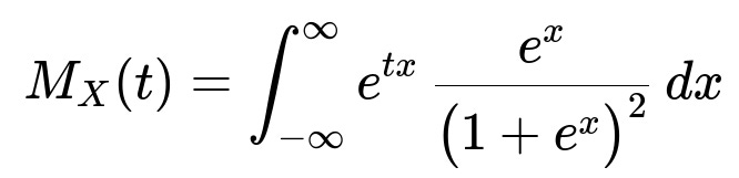
Through the substitution u = 1/(1 + e^x), one can transform this integral into a beta-function form and confirm that it converges if and only if −1 < t < 1. Hence, the mgf exists on the interval −1 < t < 1.
Expectation E(X)
To find E(X), we use the fact that E(X) = M_X'(0). One can differentiate the integral representation of M_X(t) with respect to t, then evaluate at t=0. A direct (yet somewhat intricate) integration shows that:
E(X)=0
The intuition is that the logistic density is symmetric in a log-odds sense about x=0. One may also note from the logistic distribution’s shape that it is symmetric around zero.
Variance Var(X)
We then compute the second derivative of M_X(t) at t=0. That is, Var(X) = M_X''(0) − [M_X'(0)]^2. Since M_X'(0) = 0, the variance reduces to M_X''(0). By evaluating the corresponding integral, one obtains:

Hence the logistic distribution has variance π^2/3, which is roughly 3.2899..., larger than the variance of the standard normal distribution (which is 1), indicating heavier tails.
Additional Follow-up Question: Why does the mgf converge only for −1 < t < 1?
This boils down to the exponential factor e^(t x) in the mgf and the specific shape of the logistic pdf. For large positive x, e^x/(1+ e^x)^2 behaves roughly like e^−x (since for large x, 1+ e^x ≈ e^x), but we multiply that by e^(t x). Hence, for x → +∞, the integrand behaves like e^((t−1)x), which converges if t−1 < 0, or t < 1. Similarly, for x → −∞, we get e^(t x) times e^x/(1+ e^x)^2 ~ e^((t+1)x), which converges if t+1 > 0, or t > −1. Putting these together yields −1 < t < 1.
Additional Follow-up Question: What is the relationship between the logistic distribution and logistic regression?
The logistic distribution is central to logistic regression because logistic regression models the log-odds of the probability of an event. If p is the probability of a binary outcome, then logistic regression uses the assumption:
log( p / (1 − p) ) = β_0 + β_1 x_1 + ... + β_n x_n.
The logistic function that maps real numbers to (0,1) arises exactly from inverting this log-odds relationship. Although the distribution of data points in a classification setting is not strictly “logistic,” the logistic function as a link function is the core reason the name “logistic” also appears.
Additional Follow-up Question: Does the logistic distribution have heavier or lighter tails compared to the normal distribution?
The logistic distribution has heavier tails than the normal. This is evident by looking at the tail behavior of each distribution and also by comparing their kurtosis. The logistic distribution’s variance π^2/3 is larger than 1 (which would be the variance of a standard normal). This heavier-tail property can be advantageous in certain modeling situations where outliers or extreme events are more frequent than predicted by a normal distribution.
Additional Follow-up Question: How can we confirm this result in Python numerically?
You can generate random samples from the logistic distribution and estimate the sample mean and variance to verify E(X)=0 and Var(X)=π^2/3. For example:
import numpy as np

# Generate large sample from logistic
sample_size = 10_000_000
logistic_samples = np.random.logistic(loc=0.0, scale=1.0, size=sample_size)

estimated_mean = np.mean(logistic_samples)
estimated_var = np.var(logistic_samples)

print("Estimated Mean:", estimated_mean)
print("Estimated Variance:", estimated_var)
With a sufficiently large sample, you should see the empirical mean approach 0 and the empirical variance approach π^2/3 ≈ 3.2899.
Below are additional follow-up questions
Is the logistic distribution part of the exponential family?
Yes, the logistic distribution belongs to the location-scale exponential family. An exponential family has a pdf that can be written in the form exp(θT(x) − A(θ) + h(x)), where θ is a parameter (or vector of parameters), T(x) is a sufficient statistic (or vector of sufficient statistics), and A(θ) is the log-partition function. The logistic distribution, in its standard form (location = 0, scale = 1), can be written in a shape that fits this template, although it is sometimes less commonly referred to as “exponential family” in everyday usage compared to distributions like the normal or gamma. A subtlety in practice is that while the logistic is indeed an exponential family distribution, it is a curved exponential family when one considers both location and scale parameters. This means that both parameters do not always factor in the simplest way as in canonical exponential families. Nonetheless, the logistic does share many of the convenient properties (e.g., existence of sufficient statistics for location and scale parameters).
How does the logistic distribution’s PDF differ from the normal distribution’s PDF in terms of shape, and how can that affect modeling choices?
Although both logistic and normal distributions are unimodal and symmetric about their respective means, the logistic pdf has heavier tails. The logistic pdf’s peak at the center is somewhat narrower than the normal’s peak, but it decays more slowly out in the tails. In modeling choices, these heavier tails imply that large deviations from the mean occur more frequently under a logistic distribution. If a dataset has more extreme observations than a normal model can capture, the logistic might fit better. However, if the tails are not quite that heavy, a normal model might be more appropriate. The heavier tails also influence the kurtosis, so the logistic may be a better fit when data exhibit “outlier-like” behavior. Conversely, if outliers are not expected, the normal distribution might suffice and can be simpler in certain analytical frameworks.
Given that the logistic distribution is heavier-tailed, how might that influence robust parameter estimation?
Heavier tails imply that extreme data points have a higher probability of occurring compared to a light-tailed distribution. In estimation tasks, especially if you use methods like maximum likelihood estimation (MLE), the presence of heavier tails can reduce the impact of outliers on parameter estimates compared to, for example, the normal distribution. That said, “robustness” is typically associated with distributions that have even heavier tails or with specialized estimators (e.g., M-estimators). A logistic model may be somewhat more robust than a normal-based model but it is not necessarily robust in a strict sense if the data exhibit extremely large outliers or if the distribution’s shape is significantly different from logistic. Practitioners sometimes choose even heavier-tailed distributions (like Student’s t with small degrees of freedom) to improve robustness against outliers.
What is the characteristic function of the logistic distribution, and can it be used to derive sums of logistic random variables?
The characteristic function φ_X(t) of a random variable X is E(exp(i t X)), where i is the imaginary unit. For the standard logistic distribution, the characteristic function φ_X(t) is given by a known closed-form expression involving the hyperbolic function sinh. Specifically, one way to write it is:
φ_X(t) = π t / (sinh(π t)).
This form is analogous to how the mgf was derived but now with i t instead of real t. In principle, one can use characteristic functions to analyze the distribution of sums of independent logistic random variables. However, unlike the normal distribution (where sums of normals remain normal), sums of independent logistic random variables do not remain logistic. The logistic distribution is not stable under convolution, so you do not end up with another logistic distribution for the sum. Instead, you would take the product of individual characteristic functions to get the characteristic function of the sum, and then invert it if you wanted the exact distribution.
Can we find closed-form expressions for higher-order moments of the logistic distribution beyond the second moment?
For the standard logistic distribution, the odd central moments (third, fifth, etc.) will generally be zero because the distribution is symmetric around zero. Even central moments can be expressed using integrals or known expansions involving the polygamma function or trigamma function. However, they do not have simple, well-known numeric constants like the variance does. Concretely, you can write E(X^4), E(X^6), etc. in terms of special functions, but the results tend to become increasingly complicated. In practice, the second moment (and thus variance) is often the most important for many modeling applications, so closed-form expressions for higher moments, while available, are not used as frequently.
What is the standard logistic distribution’s relationship to the logit function and how does that shape practical applications?
The logistic distribution’s cumulative distribution function (CDF) is the logistic function: F(x) = 1 / (1 + e^(-x)). The inverse of that logistic function is the logit, defined as log(p / (1−p)). This direct relationship to the logit is the reason the logistic distribution is so pivotal in logistic regression and other classification models. In practical applications, logistic regression models the logit of the probability p of a binary outcome as a linear function in the predictors. The logistic CDF then translates that log-odds value back to a probability. This connection makes the logistic distribution a natural choice for binary outcomes where the “odds” concept is intuitive and well-defined, especially in fields like epidemiology and social sciences.
If we transform a logistic random variable with a linear transformation Y = aX + b, what is the resulting distribution, and how does it scale or shift the parameters?
If X is a standard logistic random variable with pdf f_X(x) = e^x / (1 + e^x)^2, and Y = aX + b, then Y follows a logistic distribution with location parameter b and scale parameter a (assuming a > 0). Specifically, the pdf of Y becomes:
f_Y(y) = exp((y − b)/a) / [a (1 + exp((y − b)/a))^2].
Hence, a logistic random variable is closed under affine transformations in the sense that any linear shift b plus scale a yields another logistic distribution with the location b and scale a. This is analogous to how a standard normal can be turned into a general normal with mean μ and variance σ^2 by a linear transformation.
Are there any well-known limitations or pitfalls of the logistic distribution in real-world data modeling, and if so, what are possible alternatives or solutions?
One key limitation is that if your data have either extremely light tails (less frequent outliers) or extremely heavy tails (too many outliers), the logistic may not fit well. Despite having heavier tails than the normal distribution, the logistic may not be heavy enough for some data sets (like those with power-law-type tail behavior). Furthermore, if the data do not exhibit the characteristic “S”-shaped cumulative distribution when plotted on a probability scale, the logistic might be an awkward fit. In that case, one might consider:
Student’s t-distribution for heavier tails, especially when outliers are frequent.
Generalized logistic or other distributions that allow for additional shape parameters.
Extreme value distributions (e.g., Gumbel or Frechet) if the data generating process is known to be governed by maxima or minima of underlying processes.
Understanding your domain and the underlying process is crucial before selecting the logistic distribution as the model.
How does the location-scale parameterization of the logistic distribution generalize the standard logistic distribution, and how are those parameters interpreted in practice?
A general logistic distribution can be expressed as:
f(x; μ, s) = exp((x − μ)/s) / [s (1 + exp((x − μ)/s))^2],
where μ is the location parameter and s > 0 is the scale parameter. In this parameterization:
The mean of X is μ.
The variance of X is (π^2 / 3) s^2.
The heavier tails compared to a normal remain, but the scale stretches or compresses the distribution.
Interpretation-wise, μ shifts the center of symmetry of the distribution to μ, while s controls how “stretched” the distribution is (larger s means fatter tails and a wider central region). This parameterization is widely used in logistic regression, where one commonly uses the standard logistic as a baseline and adjusts for scale and location via linear predictors and other transformations.
Is there any known distribution that is more robust or heavier-tailed than the logistic for certain real-world phenomena, or is logistic always a good choice?
Many distributions are heavier-tailed than the logistic. Some examples include:
Student’s t-distribution (especially with low degrees of freedom) can be used if you suspect more extreme outliers than logistic or normal can handle.
Cauchy distribution, which is a t-distribution with 1 degree of freedom, is even heavier-tailed, but it has undefined moments (mean and variance do not exist).
In practice, logistic is not universally “the best.” It is a convenient option when working with log-odds interpretation and for moderate tail heaviness. If data exhibit extremely heavy tails or a specific structure that logistic cannot capture, you may consider alternatives. The choice always depends on empirical diagnostics (e.g., Q-Q plots, tail analysis) and domain knowledge about how the data are generated.