
ML Interview Q Series: Finding Related Topic Groups Using Graph Connected Components Analysis.

📚 Browse the full ML Interview series here.
5. There are n topics on Twitter and a notion of topics being related. If topic A is related to topic B, and topic B is related to topic C, then A is indirectly related to C. A topic group is any group of topics that are directly or indirectly related. Given an n×n adjacency matrix N, write a function to determine how many topic groups there are.
This problem was asked by Twitter - Medium.

Below is an in-depth reasoning on how to determine the number of connected components in this graph, which corresponds to how many “topic groups” there are. We will explore a Depth-First Search (DFS)/Breadth-First Search (BFS) approach and a Union-Find (Disjoint Set Union) approach. We will also consider potential pitfalls, edge cases, and multiple follow-up questions, answering them with thorough explanations.
Understanding the Graph Representation with the Adjacency Matrix
To represent a graph with n nodes using an adjacency matrix:

In an undirected graph, a “group” or “connected component” is a set of nodes where each node is reachable from any other node in that same set via some path. Counting how many connected components (or “topic groups”) exist answers the question.
Approach 1: DFS or BFS to Count Connected Components
The general idea:
Maintain a visited set or list to keep track of topics that have already been included in some discovered group.
Iterate over each topic. If a topic has not yet been visited, start a new DFS/BFS from that topic to visit every other topic reachable from it.
Mark each visited topic during the traversal.
Increment the count of connected components by one each time you initiate a new DFS/BFS on an unvisited topic.
At the end, the count of connected components (i.e. how many times you had to initiate a new DFS/BFS) is the number of topic groups.

Below is a possible Python implementation using DFS. The same concept applies if one uses BFS with a queue; the difference is only in how nodes are explored, not in the complexity or final result.
def count_topic_groups_dfs(adj_matrix):
    n = len(adj_matrix)  # Number of topics
    visited = [False] * n

    def dfs(node):
        stack = [node]
        while stack:
            current = stack.pop()
            for neighbor in range(n):
                # Check if there's an edge and if neighbor not visited
                if adj_matrix[current][neighbor] == 1 and not visited[neighbor]:
                    visited[neighbor] = True
                    stack.append(neighbor)

    group_count = 0

    for i in range(n):
        if not visited[i]:
            # We found a new connected component
            visited[i] = True
            dfs(i)
            group_count += 1

    return group_count
Explanation of the DFS approach:
We track the visited array, which starts as all False.
We iterate through each node. If a node is not visited, it triggers the discovery of a new connected component, so we increment our “group_count.”
We run a DFS from this node, using a stack (but we could just as easily use recursion). During the DFS, for each adjacent neighbor that has an edge to the current node, if it is unvisited, we mark it visited and push it to the stack.
Once the DFS returns, all nodes connected to the initial node have been marked visited. We then move on to the next node in the outer loop.
At the end, “group_count” will hold the number of connected components, i.e., the number of topic groups.
Approach 2: Union-Find (Disjoint Set Union)
An alternative strategy is to use the Disjoint Set Union-Find data structure, which can be especially efficient when dealing with repeated “is related to” queries. The Union-Find data structure maintains a collection of disjoint sets and supports two primary operations:
Union: merge two sets if they have at least one element in common.
Find: determine which set a particular element belongs to.
We can implement the algorithm:

A sample Python implementation:
def count_topic_groups_union_find(adj_matrix):
    n = len(adj_matrix)

    parent = [i for i in range(n)]  # parent[i] is the parent (or representative) of set containing i
    rank = [0]*n                   # Used for union by rank optimization

    def find(x):
        if parent[x] != x:
            parent[x] = find(parent[x])  # Path compression
        return parent[x]

    def union(x, y):
        root_x = find(x)
        root_y = find(y)
        if root_x != root_y:
            if rank[root_x] > rank[root_y]:
                parent[root_y] = root_x
            elif rank[root_x] < rank[root_y]:
                parent[root_x] = root_y
            else:
                parent[root_y] = root_x
                rank[root_x] += 1

    # Union sets for each edge
    for i in range(n):
        for j in range(i+1, n):
            if adj_matrix[i][j] == 1:
                union(i, j)

    # Find how many distinct roots
    roots = set()
    for i in range(n):
        roots.add(find(i))

    return len(roots)
Explanation of the Union-Find approach:
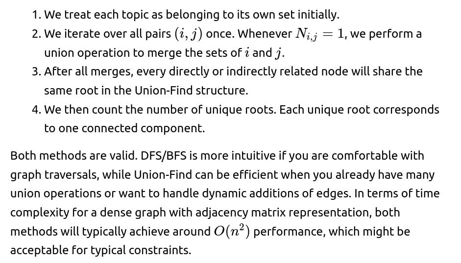

Disconnected nodes. If a node has no edges at all to any other node, it still counts as its own connected component. The iteration from i=0 to n−1 in the DFS/BFS or the separate sets in Union-Find naturally covers this scenario.
Large n. An n×n adjacency matrix can be expensive in memory when n is large (e.g. tens of thousands). For extremely large n, an adjacency list is often more efficient if the graph is sparse. The matrix-based approach is straightforward for moderate n. For very large n, one must consider memory constraints.
Indexing issues. In practice, you have to pay attention to whether your problem is 0-based or 1-based. The adjacency matrix in a Python list-of-lists is typically 0-based.
Now, below are potential follow-up questions that an interviewer might ask, along with detailed, in-depth answers. Each question is repeated verbatim in H2 format, followed by a thorough analysis.
How do you handle the case where the adjacency matrix might not be symmetric? Would the solution still work if the matrix is for a directed graph?

If “indirectly related” is meant in terms of directed paths, we need to find strongly connected components (SCCs). In that case, DFS-based approaches (Kosaraju’s or Tarjan’s algorithm) or BFS-based approaches for SCCs would be relevant.
If “indirectly related” is meant in a weakly connected sense (i.e. ignoring direction, if there is a path from one node to another by traversing edges irrespective of direction), we could symmetrize the matrix first or build an undirected graph from the directed edges. Then we count the connected components in that new undirected graph.
Hence, if the problem is truly about an undirected concept, the adjacency matrix is typically assumed to be symmetric. If it is not, either the problem is incorrectly framed for an undirected solution, or one has to reinterpret the meaning of “relation” and decide which type of connectivity (weak or strong) is relevant. The standard solution for counting connected components requires symmetrical adjacency for an undirected graph.
Can we make your DFS code recursive instead of using a stack? What are the potential issues with recursion in Python?
Yes, we can implement the DFS in a recursive style. Below is a version that uses recursion:
def count_topic_groups_dfs_recursive(adj_matrix):
    n = len(adj_matrix)
    visited = [False] * n

    def dfs(node):
        visited[node] = True
        for neighbor in range(n):
            if adj_matrix[node][neighbor] == 1 and not visited[neighbor]:
                dfs(neighbor)

    group_count = 0
    for i in range(n):
        if not visited[i]:
            dfs(i)
            group_count += 1

    return group_count
Potential issues with recursion in Python:
The default recursion limit in Python is often 1000. If n is very large or if there is a path in the graph that is extremely deep, we risk hitting a
RecursionError.While this can be mitigated by either increasing the recursion limit using
sys.setrecursionlimit()or by using an iterative approach, it is something to be aware of if the size of the graph is large.A stack-based DFS or BFS with a queue avoids the recursion limit problem but can be more verbose in code.
Why might the Union-Find approach be advantageous for this problem?
The Union-Find (Disjoint Set) approach can be advantageous when:
You want to quickly merge sets of topics without having to do a full DFS each time a new relationship is introduced.
If you have a large number of edges to process, but you do not actually need to do repeated queries of “how many connected components so far?” at intermediate steps, a single pass with union-find is quite efficient and easy to implement.
In typical interview or real-world scenarios where we get a batch of edges and we just need to know how many connected groups result from them, both DFS/BFS and Union-Find are acceptable. If you expect incremental queries over time (like repeatedly adding a new relation and then wanting the updated number of topic groups), Union-Find can be more efficient than re-running a full DFS/BFS on each addition.
What if we only wanted to list all the groups and the topics in each group instead of just counting them?
If you need the composition of each connected component, a straightforward way is to modify the DFS/BFS approach:
Instead of only keeping a visited set and an integer counter, you can also keep track of the nodes visited in each traversal.
Each time you find an unvisited node and start a DFS/BFS, you create a new list (or set) for that component, store all visited nodes from that search in it, and append it to a list of components.
A pseudocode adaptation:
def list_topic_groups_dfs(adj_matrix):
    n = len(adj_matrix)
    visited = [False]*n
    groups = []

    def dfs_collect(node, component):
        stack = [node]
        visited[node] = True
        while stack:
            current = stack.pop()
            component.append(current)
            for neighbor in range(n):
                if adj_matrix[current][neighbor] == 1 and not visited[neighbor]:
                    visited[neighbor] = True
                    stack.append(neighbor)

    for i in range(n):
        if not visited[i]:
            component = []
            dfs_collect(i, component)
            groups.append(component)

    return groups
In “groups”, each element would be a list of the nodes belonging to that connected component.
Using the Union-Find approach, you can similarly collect the components by:
Performing all unions.
Then do a pass over all nodes to find their root.
Build a dictionary from root to list of members.
The dictionary keys are the distinct roots, and the values are the lists of nodes in each group.
Could this be solved if we only had the adjacency list or edges list, rather than the adjacency matrix? What changes?
Yes, it can be solved with an adjacency list or even a list of edges. The logic is the same—both DFS/BFS and Union-Find only need to know which pairs of nodes are connected:
With an adjacency list, to do a DFS/BFS, you iterate directly over the neighbors of each node (which can be more efficient if the graph is sparse).
With a list of edges, you can do either approach: for DFS/BFS, you would first convert edges to an adjacency list structure. For Union-Find, you can directly union the endpoints of each edge.

Could parallel or distributed approaches be used here for very large Twitter topics?
Yes, for extremely large scale problems (like those that might be encountered in a real Twitter production environment), parallel or distributed graph processing frameworks (e.g. Apache Spark, GraphX, or other specialized systems) can handle connectivity computations on massive graphs. At a high level, these frameworks often break down the graph, store partitions on different nodes, and can run BFS or Union-Find in a parallel manner.
With Union-Find, a parallel implementation can use something like a MapReduce approach to do repeated passes where each node’s parent pointer is updated until stable. With BFS or DFS, one might expand a frontier of reachable nodes layer by layer, distributing the updates across multiple machines.
The fundamental concept remains the same: we want to track which topics connect to which, directly or indirectly, but the scale can make it necessary to use large-scale graph-processing frameworks.
What is the time complexity for your DFS solution? Also, what is the space complexity?
For the adjacency matrix with n topics:

Why not use a topological sort, or can a topological sort help here?
A topological sort applies to Directed Acyclic Graphs (DAGs). The concept of topological ordering doesn’t directly help us count connected components in an undirected graph. Topological sorting is about ordering vertices so all edges go from earlier to later in the order, and it is useful for tasks like dependency resolution. It doesn’t measure connectivity or grouping. Even in a directed scenario, topological sort alone will not be enough to identify strongly connected components. For strongly connected components, algorithms like Kosaraju’s or Tarjan’s are used.
Hence, topological sort is not relevant for counting how many connected (or indirectly related) topic groups are in this problem’s typical interpretation.
What if some rows in the adjacency matrix are entirely zero?
That indicates a topic that has no direct relationship to any other topic. It is effectively an isolated node. Each such topic is its own connected component if it never appears in a relation with any other node. In the DFS/BFS approach, when the algorithm checks that node, it sees no neighbors, so that node will be visited alone, increasing the connected component count by one. In the Union-Find approach, that node would never get unioned with any other node, so it remains in its own singleton set.
What if the matrix is extremely large (like tens of thousands or more)? Can the DFS approach still work with adjacency matrix representation?

How could we adapt this to a scenario where topics are being added or removed dynamically?
If topics (nodes) or edges are added or removed frequently, a plain DFS/BFS or the basic Union-Find approach might not be efficient, because you might need to recalculate large portions of the connectivity from scratch. For dynamic connectivity:

A simpler approach is to store everything in a Union-Find if the graph only adds edges (i.e., no edge removal). Union-Find can simply keep unioning sets as new edges arrive. If edges or nodes are removed, Union-Find can’t revert that easily.
In a real scenario (like Twitter topics), new relationships are likely formed as new edges. If removal is also a possibility, advanced dynamic connectivity data structures might be needed, or we might occasionally recompute from scratch when the structure changes drastically.
Any final thoughts on subtle corner cases that might confuse someone in an interview?

Another corner case might arise if the matrix includes partial data or if there is a notion of weighting edges rather than just a binary adjacency. If we had weights, the logic for “being related” might turn into a threshold-based adjacency. But the problem here uses a binary adjacency scenario, so weighting or thresholds are not relevant unless the interviewer specifically tries to branch out the conversation.

Below are additional follow-up questions
How does the approach handle real-time data streaming in a scenario where new “related” edges appear continuously?
When edges (relationships) appear in a streaming fashion, using a static DFS/BFS or Union-Find approach once at the end might no longer suffice if we want immediate or near-real-time updates on the number of topic groups. For instance, imagine a real-time Twitter feed where new “related” signals (edges) between topics are discovered constantly.
To adapt:
One option is to use an incremental Union-Find. Each time a new relationship is observed between two topics, you simply call the Union operation on those two topic indices. Because Union-Find can be updated in nearly constant time, it is well-suited to handle a stream of relationships. You keep track of the number of distinct roots (i.e. connected components) by decrementing that count whenever two previously separate connected components merge into one. This allows for quick updates without re-running a full DFS/BFS from scratch.
However, if edges can also be removed in real-time, standard Union-Find cannot easily split a set back into separate components. Handling edge deletions or node removals often requires more sophisticated data structures such as dynamic trees, Euler Tour Trees, or link-cut trees. These are more complex to implement, but they can maintain connectivity information under edge insertions and deletions with relatively efficient operations.
Potential pitfalls:
If the volume of incoming edges is extremely large, even near-constant-time union operations can add up. It is vital to maintain efficient path compression and union by rank to keep the amortized time per operation low. Also, if at any point the historical data must be reprocessed for correctness (e.g. if some edges are invalidated), a more robust dynamic graph data structure might be required.
In real-world streaming applications, memory can also be a concern. Storing a full n×n matrix is often not possible at massive scale. Instead, edges are usually stored in sparse structures (like adjacency lists) or in specialized data stores that handle streaming graph updates.
What if the adjacency matrix is extremely large but extremely sparse? Could we use a more compressed representation?
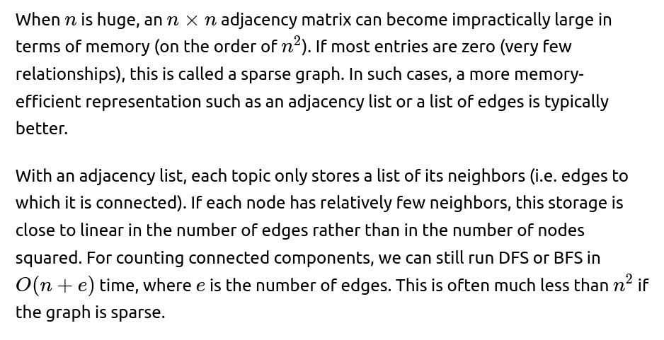
Alternatively, if the data must remain in matrix form for some reason, you can use compressed sparse row (CSR) or compressed sparse column (CSC) formats, which store only the non-zero entries. However, you would still operate your BFS/DFS or Union-Find on the unwrapped adjacency relationships. The advantage is memory savings and the possibility of faster iteration over existing edges.
Pitfalls:
• Converting a large, sparse matrix to a dense representation can lead to massive memory usage and slow processing. • If there is a sudden shift to a denser scenario (e.g., many new relationships are discovered in a short span), the chosen sparse data structure might need re-allocation, which can be costly. • Implementation complexity rises, especially if you also need parallel or distributed processing.
How can we verify correctness of the connected-component counting approach in large-scale production?
Verifying correctness typically involves multiple levels of testing and validation:
• Unit tests: With small, hand-crafted adjacency matrices (or adjacency lists), you can pre-compute the expected number of topic groups and compare the algorithm’s output. Examples:
A disconnected matrix (diagonal or entirely zero except for self-loops) should produce n connected components.
A fully connected matrix (every off-diagonal entry is 1) should produce 1 connected component.
Several intermediate patterns with known groupings.
• Integration tests: In a bigger system, feed the adjacency matrix from the actual pipeline or data store. Compare the results with a known partial or sample dataset. This might involve storing a snapshot of the matrix or edges in a test environment.
• Random tests: For large-scale verification, generate random adjacency structures with known properties (e.g., known block diagonal structure that artificially segments the graph). Then confirm the algorithm’s output matches the expected number of components.
• Real-time checks: In a streaming or real-time scenario, if feasible, compare the incremental approach’s result (e.g. the Union-Find ongoing merge count) with a full offline BFS/DFS approach done at some interval to ensure they match.
Pitfalls:
• Even small mistakes in indexing or ignoring the symmetry assumption can lead to incorrect group counts. • Race conditions or concurrency issues in distributed environments can corrupt the adjacency representation or union-find data structure. • Missing or invalid data can cause the algorithm to skip certain edges, leading to an underestimation of the number of connections.
Could we do a multi-threaded BFS or DFS to speed up the computation of connected components using an adjacency matrix?
Yes, multi-threading (or parallelism) can help when n is large, and each node’s search is independent once you decide to start a new component exploration. However, the implementation needs careful synchronization:
• One approach is to split the nodes among multiple threads. Each thread runs a DFS/BFS on unvisited nodes. When a thread finds an unvisited node, it performs the traversal and marks all reachable nodes as visited. • You need to ensure that no two threads simultaneously start a traversal for the same node. Typically, you keep a shared visited array that is updated atomically or under locks. • Union-Find can also be parallelized. Each edge insertion can be handled in separate threads, though again you need atomic or lock-based updates to the parent pointers. There are known parallel Union-Find algorithms that handle concurrency with minimal locking.
Pitfalls:
• Overhead due to synchronization might negate the speed benefits if n is not large enough. • Load balancing: some components might be much bigger than others, causing certain threads to handle huge traversals while others remain idle. • Implementation complexity: ensuring correctness and avoiding data races can be tricky.
In many production systems, a distributed graph processing framework (like Spark, GraphX, or Pregel-like systems) is often chosen over manual multi-threading because it handles many concurrency and partitioning details.
How might the design of the adjacency matrix change if topics come from diverse domains (e.g., multi-lingual or multi-modal data)?
In real-world social networks, “topics” might be multi-lingual or come from different data modalities (e.g., text, images, videos). The adjacency matrix might then represent relationships across these different contexts. For instance, a relationship might mean “topic in language A is semantically related to topic in language B due to a translation or correlation.” This can complicate how edges are determined.
In practice: • One might define a rule-based or ML-based approach that extracts edges by measuring similarity or correlation across different languages or modalities. • The adjacency matrix might become extremely large, as it spans multiple categories or domains of topics. • Some edges could be assigned different weights or confidence levels, suggesting the possibility of thresholding (only edges above a certain confidence become “1”).
Pitfalls:
• Defining what “related” means can be subjective and might require domain-specific thresholds. • Errors in cross-lingual or multi-modal similarity detection can introduce spurious edges or miss valid ones, potentially merging separate topic groups or leaving them split incorrectly. • Handling partial overlap or out-of-vocabulary scenarios can reduce the adjacency matrix’s reliability.
How can we incorporate weights or similarity scores into the grouping? Is it still just a connected components problem?
If “relatedness” is binary, we do a straightforward connected components approach. However, in many real-world scenarios, there is a weight or a confidence measure that expresses how strongly two topics are related. One might have a matrix of continuous similarity scores. Converting these scores into edges typically involves choosing a threshold: any similarity above that threshold is considered an edge.
If the threshold is too high, you get too many components (the graph is very fragmented). If the threshold is too low, you might get one giant component. Tuning that threshold can be a challenge.
Alternative approaches:
• Clustering algorithms like spectral clustering or hierarchical clustering can operate on continuous similarity matrices. They do not merely produce connected components but group topics based on overall similarity structure. • A threshold-based approach is the simplest extension for “weighted adjacency” to remain in the connected components framework.
Pitfalls:
• Setting a single global threshold might not be appropriate if the distribution of similarity scores varies by topic domain. • If edges represent trust or confidence, you might want a more nuanced approach that incorporates additional metadata rather than a simple threshold. • Weighted graphs can have advanced definitions of connectivity, such as “strongest path” connectivity. But that goes beyond standard binary connected components.
What happens if the adjacency matrix has partial or missing data?
In real-world datasets, you might lack complete knowledge of whether certain topics are related. For instance, some cells in the adjacency matrix might be unknown. You could represent that with a special marker (e.g., -1) or some null value.
Approaches to handle missing data:
• Ignore unknown entries and treat them as 0 (no edge). This might cause underestimation of the number of edges, resulting in more disconnected components. • Use probabilistic inference to estimate whether the unknown entry should be 1 or 0, effectively imputing the missing data. That usually involves domain knowledge or a machine learning model that can predict the likelihood of a relation. • Perform upper and lower bound analyses: assume all unknown entries are 0 to get a minimum connectivity scenario, and assume they are 1 to get a maximum connectivity scenario. This might bracket the possible range of connected components.
Pitfalls:
• If too many entries are unknown, the notion of connectivity becomes very uncertain. • Imputing missing data incorrectly can drastically change the connectivity count if it introduces or removes many edges. • Partial data can create illusions of isolation: some topics might appear disconnected only because their potential connections are unknown, not necessarily absent.
If we need to find the largest or smallest connected component, how do we adapt these approaches?
To identify the largest or smallest components after finding connected components, you can store component sizes during or after the connectivity procedure:
Using DFS/BFS: • Each time you discover a new component, keep a running count of how many nodes you visit in that DFS/BFS. Store that count. • Compare across all components to determine the maximum or minimum size (or list them all for a more general analysis).
Using Union-Find: • After all unions are done, iterate through each node, find its root, and increment a counter in a dictionary keyed by the root. • Then examine the dictionary values to find the largest or smallest group.
Pitfalls:
• Make sure to handle isolated nodes. Their component size is 1. • In a scenario with merges in a streaming context, you might keep track incrementally of each component’s size. Each union merges two sets; you add their sizes and update the count for the new root. • If the graph has many medium-sized components, storing all sizes might be large in memory. But typically, a dictionary of size nn is feasible if you only store one integer per node or one integer per root.
How can load-balancing be approached in a distributed environment if some components are disproportionately large?
In large social network graphs (like Twitter’s real data), it’s common to have a “giant” component plus many tiny ones. A naive distributed BFS might get stuck if one partition contains the majority of edges. Load-balancing challenges include:
• Dynamic partitioning strategies: some systems re-balance the graph partitions at runtime by moving nodes or edges to different machines based on the current BFS frontier. • Random partitioning: sometimes, simply distributing edges randomly across machines can help average out the load, though it may increase cross-node communication. • Graph partitioning heuristics (e.g., METIS or other specialized partitioners) attempt to minimize cut edges. This can reduce cross-partition traffic but might still result in skewed BFS expansions if a single large component is heavily localized.
Pitfalls:
• Over-partitioning can create overhead in communication and synchronization across too many machines. • Maintaining a globally consistent visited set in BFS or maintaining union-find parents across multiple machines is non-trivial, often requiring message passing or shared state management. • There might be diminishing returns if the overhead of coordination outweighs the parallel gains.
How do we handle ambiguous or conflicting relationship information that might exist in the adjacency matrix?
In practical settings, especially with user-generated content or noisy data, different sources might disagree about whether topic A is related to topic B. One source says 1, another says 0. Some systems might have multiple adjacency matrices or reliability scores for each edge.
Possible resolutions:
• Majority vote: If enough sources claim the relationship is valid, set it to 1; otherwise 0. • Weighted or probabilistic edges: Keep a probability or weight for each edge and adopt a threshold. • Multi-layer graphs: Instead of a single adjacency matrix, store multiple layers, each from a different source or different confidence band, and run connectivity analysis on each layer or a combined graph.
Pitfalls:
• Inconsistent data can lead to contradictory edges (some portion of the data says they are connected, some not). This might cause confusion if you want a single, definitive connected components count. • Combining data from multiple sources might artificially inflate connections, merging distinct communities. • Maintaining transparency in how edges were decided (which sources override which) can complicate the data pipeline and the final connected components result.