
ML Interview Q Series: Gambler's Ruin: Calculating the Probability of Reaching a Target Before Ruin.
Browse all the Probability Interview Questions here.
Imagine a scenario in which you have 30 dollars to start. Each time you flip a coin, you either gain 1 dollar if it’s heads or lose 1 dollar if it’s tails. You continue flipping until your money either drops to 0 or climbs to 100 dollars. What is the probability of reaching 100 dollars before hitting 0?
Comprehensive Explanation
This question is a classic instance of the “Gambler’s Ruin” problem. You have an initial amount of money (30 dollars) and an absorbing boundary at 0 dollars (where you lose everything) and at 100 dollars (the goal). Each coin toss adds or subtracts 1 dollar, depending on whether it’s heads or tails. With a fair coin, the probability of heads is 0.5, and the probability of tails is 0.5.
Underlying Markov Chain Perspective
The process can be seen as a Markov chain, where each state is an integer amount of money you hold (from 0 up to 100). States 0 and 100 are absorbing states because once you reach either, you remain there. At each intermediate state i, you have transitions to i+1 or i-1 with probability 0.5.
Core Mathematical Formula (Fair Coin)
When the coin is fair (probability p = 0.5), an important result from gambler’s ruin theory is that the probability of eventually reaching the upper boundary N before dropping to 0, starting at some initial i, is simply i/N. Here, i is your initial amount, and N is your target.
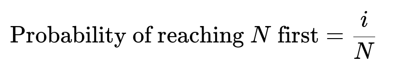
In this question, i = 30 and N = 100, so the probability that you reach 100 dollars first is 30/100 = 0.3.
Below is a deeper explanation of each variable inline:
i is the initial money (30).
N is the winning threshold (100).
p is the probability of winning 1 dollar each coin toss (0.5 for a fair coin).
q = 1 - p (also 0.5 for a fair coin).
Core Mathematical Formula (Biased Coin)
If the coin is not fair, the general formula is:
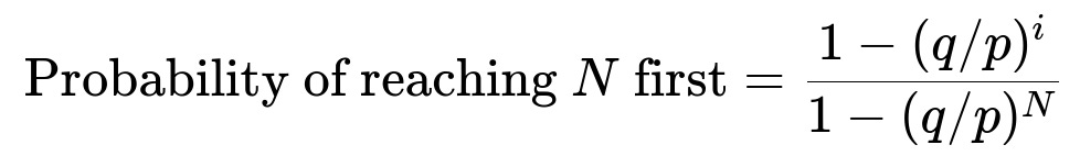
Where p is the probability of winning a dollar each time, q = 1 - p, i is the starting money, and N is the target. When p = 0.5, q/p = 1, so this expression reduces to i/N.
Simulation Approach in Python
A straightforward way to verify this result is by simulation. The code below repeatedly simulates the coin flips, tracks the money until it hits 0 or 100, and estimates the probability by counting how many times 100 is reached.
import random

def simulate_gambler_ruin(p=0.5, initial_money=30, target=100, trials=1_000_00):
    wins = 0
    for _ in range(trials):
        money = initial_money
        while 0 < money < target:
            flip = random.random()
            if flip < p:
                money += 1
            else:
                money -= 1
        if money == target:
            wins += 1
    return wins / trials

# Example usage:
estimated_probability = simulate_gambler_ruin()
print("Estimated Probability of Reaching 100 Dollars:", estimated_probability)
If you run this many times (in the order of hundreds of thousands or millions of trials), you should see the estimate settling close to 0.3.
Possible Follow-up Questions
How does the formula i/N arise for a fair coin?
The derivation exploits the fact that when p = q, the expected net change over each flip is zero. The probability distribution of hitting either boundary can be derived by solving a system of linear equations or by using martingale arguments. For a fair game, the solution simplifies to a linear function in the initial amount i.
When p = 0.5, the ratio q/p is 1. In the more general expression with the factor (q/p) raised to certain powers, substituting (q/p) = 1 collapses everything to i/N.
What happens if the coin is biased?
If p is not 0.5, the probability of eventually reaching N changes to the formula (1 - (q/p)^{i}) / (1 - (q/p)^{N}). For instance, if p > 0.5, it becomes more likely to reach 100 than to drop to 0. Conversely, if p < 0.5, the chance of ruin increases.
Could you interpret this through a Markov chain approach?
Each state 1, 2, 3, …, 99 transitions to i+1 with probability p and i-1 with probability q. States 0 and 100 are absorbing. The transition matrix has a special tridiagonal form with absorbing boundaries. Finding the probability of eventually reaching state 100 is equivalent to determining the fundamental matrix of the absorbing Markov chain, or solving boundary value problems in discrete space. The gambler’s ruin formula emerges as the closed-form solution.
Is there an intuitive explanation of why the answer is 0.3 for the fair coin scenario?
One intuitive explanation is symmetry. If the game is fair, you expect to “randomly walk” between 0 and 100. Because you start at 30, you effectively have 30 “steps” behind you (toward 0) and 70 “steps” to go before hitting 100. Under symmetry assumptions, your fraction of the total distance (30 out of 100) is the fraction of times you would, on average, make it to 100 before slipping to 0.
What is the expected time (number of flips) before the game ends?
For a fair game starting at i, the expected time to absorption can be computed using classic gambler’s ruin analysis. The result for the fair case (p = 0.5) starting at i, with boundaries 0 and N, turns out to be i * (N - i). In this scenario, 30 * (100 - 30) = 30 * 70 = 2100 flips on average. If the coin were biased, the expression would differ.
What if we apply different increments or decrements for each outcome?
If heads gives you something other than +1, or if tails subtracts a different amount, the Markov chain states could still be analyzed similarly, but the transition probabilities and step sizes would change. The resulting boundary-hitting probabilities would require solving a more generalized difference equation. The principle remains similar, but the formula becomes more complex.
Do real-world casinos or trading systems follow this pattern?
Many real-world betting games have a house edge, meaning p < 0.5 effectively, which shifts the probabilities so that the gambler’s chance of ruin is higher. Similarly, in trading, transaction fees introduce a tilt away from fairness. Although real-world scenarios have additional complexities such as changing probabilities or partial bets, the gambler’s ruin model provides a rough baseline understanding of risk and reward in sequential betting.
These thorough explanations and follow-up discussions cover the core theoretical aspects, practical simulation, and potential variations that might arise in a real-world or interview setting.
Below are additional follow-up questions
How does the Optional Stopping Theorem relate to gambler’s ruin?
One way to analyze gambler’s ruin is through the lens of the Optional Stopping Theorem (OST). OST states that if you have a martingale (a fair game with zero expected gain) and a stopping time (the time when you decide to stop playing), under certain conditions, the expected value of the martingale at that stopping time is equal to its initial value.
For gambler’s ruin, consider the fair coin setting where the expected increment per toss is zero. You can define a process X_n as your current money after n flips. Since each flip is fair, X_n is a martingale. The time to reach 0 or 100 is your stopping time. OST implies that the expected value at the stopping time should be the same as the initial value, provided the game ends in finite time and you do not violate the regularity conditions (like unbounded stopping times). Although you eventually do reach an absorbing boundary (guaranteed by the rules of random walks in finite states), verifying conditions to rigorously apply OST can be subtle. The direct application of OST also highlights why, for a fair coin, the average outcome remains the same over the process, leading to the simple formula i/N for the probability of eventually reaching 100.
Pitfall to watch out for: If the stopping time is not guaranteed to happen in a bounded time (for instance, in an unbounded random walk with no absorbing boundaries), applying OST can be more delicate or invalid if certain conditions (e.g., integrable stopping time) are not met.
What if the coin tosses are correlated rather than independent?
Most gambler’s ruin derivations hinge on the assumption of independent flips. If flips become positively or negatively correlated, then standard closed-form formulas break down because the probability of transitioning from one state to another depends not only on the current state but also on previous states.
For example:
Positive correlation might mean a run of heads is more likely to be followed by another head.
Negative correlation might mean that after a few heads, tails become more likely.
In such scenarios, the Markov property no longer strictly holds, and analyzing the chain of states is more involved. You might resort to techniques such as:
Extending the state space to include the memory of previous outcomes.
Using advanced Markov Chain Monte Carlo methods or direct simulation to estimate probabilities.
Pitfall to watch out for: Misapplying the standard gambler’s ruin formula when correlation exists can lead to incorrect conclusions, because those formulas explicitly assume each flip is an i.i.d. Bernoulli trial.
How does the result change if the gambler adjusts the bet size dynamically?
In the classical formulation, each flip changes the amount of money by a fixed increment (±1). If the gambler can vary the bet size at each flip—say, wagering a fraction of the current bankroll—the mathematical model shifts significantly. This is akin to a Kelly criterion strategy or a variable betting scheme.
Such dynamic strategies complicate the analysis because:
The state transition depends on the gambler’s chosen action at each step.
The random walk is no longer a simple ±1 step process.
The probability of ruin and the expected time to ruin must be derived from a higher-dimensional state that includes both the gambler’s capital and the gambler’s bet size decision.
Pitfall to watch out for: It’s easy to incorrectly treat dynamic betting as equivalent to fixed-step gambler’s ruin. In reality, dynamic strategies require a separate approach or a more complex difference equation.
Could we incorporate transaction costs or a “tax” on each flip?
Introducing a small cost on each flip (like a fraction of a dollar every time you play) means that even if you win the flip, you gain slightly less than 1 dollar, and if you lose, you lose 1 dollar plus the cost. This effectively biases the game against you because the expected net is now negative.
Let’s assume each flip costs c dollars. Then:
Heads might yield +1 - c dollars.
Tails might yield -1 - c dollars.
In that case, the standard gambler’s ruin formula does not directly apply. You would need to re-derive probabilities or rely on simulations to see how quickly the incremental negative drift from the cost c drives your bankroll toward 0.
Pitfall to watch out for: Even a tiny cost per flip can drastically shift the probability of ruin when the number of flips becomes large. If the analysis is done without accounting for these transaction costs, the real-world outcomes might be much worse for the gambler than the idealized model suggests.
Is there a possibility of “infinite oscillation” in theory, and how do we address that?
In an infinite random walk without absorbing boundaries, there is a theoretical possibility that you wander around indefinitely. However, gambler’s ruin imposes absorbing boundaries at 0 and 100, making sure you eventually end at one boundary or the other. That is why the game ends almost surely.
In the continuous-time or infinite-range random walk scenario (no upper bound), it might take a very long time to come close to 0 for the first time, but as soon as you implement a hard boundary at 0 (ruin), eventually you are absorbed with probability 1. This is due to the properties of unbiased random walks in finite discrete state spaces.
Pitfall to watch out for: Confusion may arise if someone tries to apply gambler’s ruin logic to an infinite-range random walk with no boundary at the top. In that scenario, you do not have a guaranteed stopping time unless some other event triggers it. Always confirm that your random walk or Markov chain is truly bounded by absorbing barriers before applying gambler’s ruin formulas.
Can this concept be extended to more than two absorbing boundaries?
Yes. A generalized version of the gambler’s ruin problem involves multiple absorbing boundaries. For instance, imagine a scenario with boundaries at 0, 100, and 200. You start with 30, but if you ever drop to 0 you lose, if you ever climb to 100 you achieve one outcome, and if you climb to 200 you achieve a different outcome. In such a setup, the analysis would revolve around finding the probabilities of absorption at 0, 100, or 200.
One approach uses Markov chains with multiple absorbing states. You would set up transition probabilities for going from i to i+1 or i-1 and solve the corresponding system of linear equations for absorption probabilities. Each boundary condition is of the form that once you hit that boundary, you remain there with probability 1.
Pitfall to watch out for: If the system is not carefully modeled, or if the random walk transitions are not purely ±1, you can misapply the simpler gambler’s ruin formula. Extending gambler’s ruin to multiple absorbing states can be done analytically, but it typically requires more involved algebra or matrix methods.
How does the gambler’s ruin concept apply in reinforcement learning contexts?
Reinforcement learning (RL) can be thought of as an agent moving through states and receiving rewards. A gambler’s ruin model might appear in an RL environment if:
The state variable is the agent’s “capital” or resource count.
The environment transitions up or down in capital based on actions (which might be analogous to coin flips or probabilities).
When designing RL experiments, you may want the agent to learn an optimal policy to avoid ruin and reach a target resource level. One difference from classical gambler’s ruin is that in RL, the agent’s policy might adapt over time, altering transition probabilities if it can choose among multiple actions.
Pitfall to watch out for: A direct application of gambler’s ruin assumes you have no control over the probability (it’s a coin toss), whereas RL typically involves an agent selecting actions that can change transition dynamics. This means standard gambler’s ruin formulas only apply if the environment is truly stateless or if the policy cannot affect the outcome probabilities.
What if the increments are random in size, not just ±1?
Instead of winning or losing exactly 1 dollar, suppose you draw from a distribution of possible gains or losses each flip. For example, you gain or lose a random integer amount from 1 to 5, with some probability distribution. This variation is known as a random step size. You still have absorbing boundaries at 0 and 100, but each step can jump you multiple dollars in a single move.
Analyzing this situation requires:
Setting up a system of equations where the transition probability from state i to state j is governed by the distribution of step sizes.
Determining for each possible jump how likely it is to land exactly on or below 0 (ruin) or meet or exceed 100 (win).
Pitfall to watch out for: If the random step can exceed the boundary in a single jump, you need to handle scenarios where you effectively “overshoot” the boundary. You have to decide what it means if you jump beyond 100. Some approaches treat 100 as an immediate absorbing state once you cross it, others might force you to “bounce back.” The interpretation changes the probability calculation.