ML Interview Q Series: Gaussian Mixture Models for Fraudulent Transaction Anomaly Detection

📚 Browse the full ML Interview series here.

Say we are using a Gaussian Mixture Model (GMM) for anomaly detection on fraudulent transactions to classify incoming transactions into K classes. Describe the model setup formulaically and how to evaluate the posterior probabilities and log likelihood. How can we determine if a new transaction should be deemed fraudulent?

The Gaussian Mixture Model (GMM) uses a mixture of multivariate Gaussians with mixing coefficients to model the probability distribution of data. Each Gaussian in the mixture is associated with a mean vector and covariance matrix, and we fit these parameters using the Expectation-Maximization (EM) algorithm. Once trained, we obtain posterior probabilities that indicate how likely it is that a transaction belongs to each Gaussian component. For anomaly detection in fraud settings, if the likelihood of a new transaction under the GMM is too low or if it does not fit well into any of the learned mixture components (i.e., posterior probability for all components is very low), we flag it as fraudulent.

Model Setup

We consider a dataset of transaction feature vectors in a D-dimensional space. A GMM with K components is defined by:

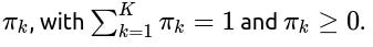
Mixing coefficients for each component, denoted as

• 

  For a transaction feature vector x, the GMM density is given by

  

  The multivariate Gaussian density for component k is

  

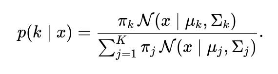
  Posterior Probabilities

  After model parameters are learned (for instance, via EM), we can compute the posterior probability that an observed point xx belongs to component k as

  

  These posterior probabilities are used to classify a transaction into the most likely Gaussian component or to compute an overall likelihood.

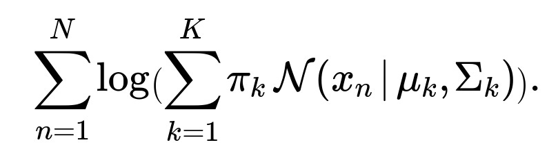
  Log-Likelihood

  Given a set of N transactions {x1,x2,…,xN}, we can evaluate the log-likelihood of the dataset under the GMM as

  

  This log-likelihood is often used during training (the EM algorithm maximizes it), and once the model is trained, the log-likelihood (or likelihood) can be used for assessing how well new transactions fit into the learned distribution.

  Determining Fraudulent Transactions

  A common practical strategy in anomaly detection with GMMs is to set a threshold on the log-likelihood or to examine how a new transaction’s posterior probability distribution compares to typical transactions. If the overall likelihood p(x) is too low or if there is no strong membership to any single component (e.g., none of the p(k∣x) are high, or they are all very small relative to typical in-distribution data), we can declare the transaction as “fraudulent.” In practice, one might set a threshold by analyzing training data or a separate validation set with known normal vs. fraudulent examples.

  Example Code Snippet

  import numpy as np
  from sklearn.mixture import GaussianMixture
  
  # Suppose X_train is your training data with shape (N, D).
  gmm = GaussianMixture(n_components=K, covariance_type='full', max_iter=100, random_state=42)
  gmm.fit(X_train)
  
  # For a new transaction x_new (shape (1, D))
  log_prob = gmm.score_samples(x_new)  # log-likelihood under the model
  # If log_prob is below some threshold, label as fraudulent
  threshold = -50.0  # Example threshold set by validation
  if log_prob < threshold:
      print("Likely Fraudulent")
  else:
      print("Likely Normal")
  
  # For posterior probabilities
  posterior_probs = gmm.predict_proba(x_new)
  # If none of the posterior_probs are sufficiently high, flag as fraudulent
  if np.max(posterior_probs) < 0.1:
      print("Likely Fraudulent")
  else:
      print("Likely Normal")
  

  Potential Follow-Up Questions and Answers

How to choose K?

In practice, you can use techniques such as the Bayesian Information Criterion (BIC) or the Akaike Information Criterion (AIC) to compare models with different values of K and select the one that yields a good balance of model fit and complexity. You could also do cross-validation to see how different K values generalize.

How to handle high-dimensional data?

In very high dimensions, full covariance estimates can be unstable or prone to overfitting. Options include using diagonal or tied-covariance settings, regularizing the covariances, or performing dimensionality reduction (e.g., PCA) prior to fitting the GMM.

What is the difference between GMM for clustering vs. anomaly detection?

For clustering, we usually want each component to represent a cluster of “typical” samples in the data. For anomaly detection, we additionally focus on how far a point’s distribution-based scores fall outside the normal range. The same GMM can be used for both if carefully tuned, but the thresholding step is specific to anomaly detection.

Why use posterior probability vs. log-likelihood for anomaly detection?

Log-likelihood is a global measure of how well a sample fits the overall mixture model. Posterior probability for a specific component informs which cluster best explains the data. Both can indicate anomalies: low log-likelihood implies none of the mixture components can explain the data well, while a lack of a strong posterior membership means the data point does not belong confidently to any learned component.

How does the EM algorithm estimate the parameters?

In the E-step, the algorithm computes the expected component assignments (posterior probabilities). In the M-step, it updates the component parameters (means, covariances, and mixing coefficients) to maximize the log-likelihood given these expected assignments. This process iterates until convergence of the log-likelihood.

How to set the threshold for anomaly detection?

If you have labeled data for normal and fraudulent transactions, you can tune the threshold to maximize metrics such as F1-score, precision-recall, or area under the ROC curve. If you only have normal data, you can set a quantile-based threshold (e.g., transactions whose log-likelihood fall below the 1st percentile in a validation set are deemed anomalies).

How to interpret the covariance structures?

Large covariance values imply that the GMM cluster allows for broad variation in that dimension. If certain components have tight covariances, they specialize in highly consistent (low-variance) features. During fraud detection, anomalies sometimes appear in regions of the feature space with little data coverage, so those points have low likelihood under all mixture components.

How do you scale this in real-world streaming or near real-time settings? You can train the GMM in batches or incrementally. Some libraries support partial fits. For real-time detection, once the model is trained, computing the likelihood or posterior for each new point is fast. If you have continuous changes in data distribution, you might periodically update or retrain the GMM.

How robust is GMM-based anomaly detection to outliers in the training data? Outliers can skew the parameter estimates, especially covariance matrices. Strategies for improved robustness include using robust covariance estimators, regularization, or explicit outlier filtering before final model training.

These details demonstrate how to set up the GMM, compute posterior probabilities, log likelihoods, and use them for fraud detection by thresholding.