ML Interview Q Series: Gaussian Mixture Models for Fraudulent Transaction Anomaly Detection

📚 Browse the full ML Interview series here.

39. "Say we are using a Gaussian Mixture Model (GMM) for anomaly detection on fraudulent transactions to classify incoming transactions into K classes. Describe the model setup, how to evaluate posterior probabilities and log likelihood, and how to determine if a new transaction is fraudulent."

This problem was asked by Stripe (HARD).

Model Setup for a Gaussian Mixture Model begins with the notion that transaction data can be represented as samples from a mixture of different Gaussian distributions. Each Gaussian distribution corresponds to one of the K classes. The mixture model assumes that the observed data is generated by first sampling one of the K components according to a prior mixing probability, then generating the data from the corresponding Gaussian distribution. When applying this to fraud detection, one can interpret the fitted GMM as representing the normal modes of transaction behaviors (or a combination of normal + fraudulent transaction behaviors, if the historical data contains both kinds of transactions). Each class in the GMM is typically represented by a mean vector and a covariance matrix, along with a prior probability (also called mixing coefficient) for that class.

The parameters of the GMM are estimated using the Expectation-Maximization (EM) algorithm. In the E-step, we compute the expected cluster assignments (responsibilities) for each sample based on the current parameter estimates. In the M-step, we update the parameters (means, covariances, mixing coefficients) using those responsibilities. Iterating these two steps converges to a local maximum of the likelihood.

When evaluating the Log-Likelihood, we compute the logarithm of the probability of the data under the current model parameters. The log-likelihood is a sum (or average) of the log probabilities of each data point. The GMM log-likelihood is then maximized during EM to find the best parameter estimates. A higher log-likelihood generally indicates a better fit to the data.

Determining if a new transaction is fraudulent involves fitting the GMM to historical transaction data and learning the expected distribution of “normal” transactions. If the mixture is specifically modeled to capture normal classes, then anomalous points appear as low-probability outliers under the model. When a new transaction arrives, its likelihood under each Gaussian component can be calculated, and a final mixture-likelihood is computed by combining the per-component likelihoods weighted by the component priors. If that likelihood is suspiciously low (compared to a threshold chosen based on a desired false positive/false negative trade-off), the transaction is flagged as potentially fraudulent. Alternatively, one can also look at how the posterior distribution of responsibilities is allocated; if the transaction does not match any of the learned components (i.e., belongs nowhere with high probability), that is another sign of anomaly.

A practical approach can be: (1) estimate the GMM parameters from training data believed to be primarily normal; (2) compute an anomaly score for each new transaction as the negative log-likelihood under the trained mixture model; and (3) declare those transactions exceeding a certain threshold as fraud.

Explanations of the underlying reasoning can be made precise mathematically. One can write the mixture PDF for a transaction feature vector xx as a sum of component densities scaled by their mixing coefficients, then derive the posterior responsibilities using Bayes’ rule. By examining the magnitude of that mixture density for new transactions, one can decide whether it is in line with previously observed patterns (normal) or far from those modes (fraudulent).

In more detail:

Estimation of Model Parameters

Posterior Probability Calculation

Given an observation x and a set of parameters for the mixture components, the posterior probability (or responsibility) that component k generated x is

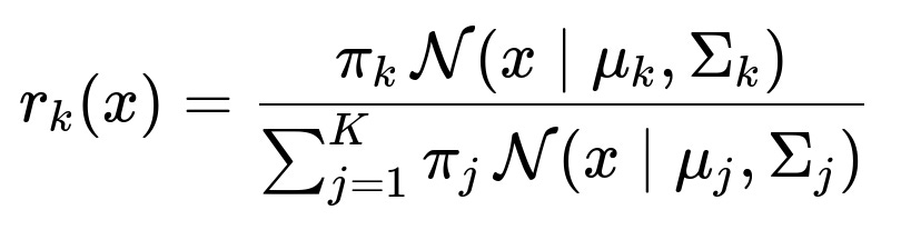
This expression is derived using Bayes’ theorem, where the numerator is the prior probability of class k multiplied by the likelihood of x under that class’s Gaussian distribution, and the denominator ensures normalization across all classes.

Log-Likelihood of the GMM

The log-likelihood for a set of N observations is the sum of the log of the mixture PDF:

Examples and Considerations

An intuitive Python code snippet with scikit-learn might look like the following:

import numpy as np
from sklearn.mixture import GaussianMixture

# Suppose we have training data in X_train
X_train = ...  # your features for past transactions

# Choose the number of components K
gmm = GaussianMixture(n_components=K, covariance_type='full', random_state=42)
gmm.fit(X_train)

# To get the per-sample log-likelihood of each training point:
train_log_probs = gmm.score_samples(X_train)  # log probabilities per sample

# Suppose we have a new transaction x_new
x_new = np.array([...])  # feature vector for the new transaction
x_new = x_new.reshape(1, -1)  # scikit-learn expects 2D

# Compute log probability
log_prob_new = gmm.score_samples(x_new)  # returns an array with one element
prob_new = np.exp(log_prob_new)  # convert log-prob to prob

# Decide if fraudulent
threshold = ...  # some chosen threshold
if prob_new < threshold:
    print("Flag as fraudulent")
else:
    print("Likely normal")

One must keep in mind that the threshold setting can make a big difference in practical fraud detection. Too low a threshold may miss a lot of fraudulent transactions (false negatives). Too high a threshold may cause many normal transactions to be flagged (false positives).

There are several subtle points to consider in real-world implementations. If fraud transactions are very rare, the overall data distribution may not capture them well through a standard GMM. In such cases, modeling normal data primarily and then using a one-sided anomaly detection approach can be more effective, or explicitly modeling a “fraud component” might be considered if there is enough labeled fraudulent data to fit such a component.

Possible Follow-up Question: "How would you handle severely imbalanced datasets where the fraction of fraudulent transactions is extremely small?"

In a practical setting, the dataset may be highly skewed, with normal transactions vastly outnumbering fraudulent ones. One strategy is to fit a GMM primarily on normal data only, making the assumption that the model captures typical transaction behavior. Any transaction that falls well outside the typical ranges is flagged as fraud. This approach relies on selecting a threshold that identifies anomalies sufficiently well. It can also be useful to employ techniques like oversampling the minority class (fraud) or undersampling the majority class, though these methods must be used with care because oversampling can artificially inflate the importance of limited fraud samples. Another option is to do a specialized anomaly detection technique such as One-Class SVM or Isolation Forest if the GMM approach fails to capture the complexities of the normal distribution.

Possible Follow-up Question: "How do you decide on the number of components K in your GMM for fraud detection?"

One approach is to use model selection criteria like the Bayesian Information Criterion (BIC) or the Akaike Information Criterion (AIC). In practice, one can train multiple GMMs with different K values, compute these information criteria, and choose the model that yields the best trade-off between goodness of fit and model complexity. Alternatively, you can use cross-validation on a validation set to see which K best separates normal transactions from known fraudulent transactions, if labeled examples exist.

Possible Follow-up Question: "What if the covariance matrices become singular or nearly singular?"

This can happen if there are too few data points to estimate a full covariance matrix for each component or if the data in a component lies on a lower-dimensional manifold. One common mitigation is to regularize the covariance matrices by adding a small diagonal term to ensure invertibility. In scikit-learn, specifying a non-zero reg_covar parameter in GaussianMixture can prevent numerical issues. Another approach is to use a more constrained model like a diagonal covariance structure if the dimensionality is high, thereby reducing the number of parameters to estimate.

Possible Follow-up Question: "How do you interpret posterior probabilities for fraud detection?"

The posterior probabilities (responsibilities) indicate how likely each transaction is explained by each Gaussian component in the mixture. In a straightforward anomaly detection setting, if the mixture is mostly modeling normal classes, one might find that a fraudulent transaction does not fit well in any of the learned clusters. This situation can be recognized by a low overall mixture density value. One can also observe which component’s posterior probability is highest for the transaction and see if that is consistent with a normal class. If the posterior for all classes is very small, that transaction is likely fraudulent.

Possible Follow-up Question: "How do you handle high-dimensional data in a GMM for fraud detection?"

High-dimensional data poses several challenges, including difficulty accurately estimating covariance matrices. If the dimensionality is extremely large compared to the number of data points, the covariance matrix for each component can become ill-conditioned. Possible solutions include using a diagonal or tied covariance structure, applying dimensionality reduction techniques such as PCA before fitting the GMM, or employing a regularization approach that constrains the covariance estimates.

Possible Follow-up Question: "How might you compare GMM-based anomaly detection to other approaches such as Isolation Forest or Autoencoder-based anomaly detection?"

When comparing GMM to alternatives, one considers data dimensionality, the presence of distinct modes, the shape of the distributions, and whether enough fraud data is available for a purely supervised approach. GMM can provide explicit probability estimates and interpretability in terms of cluster membership, but it makes assumptions about the data being drawn from Gaussian distributions. Isolation Forest or Autoencoders can be better at capturing more complex, non-Gaussian data. In practice, performance is often validated empirically, by comparing metrics like precision, recall, and ROC curves on known fraud examples.

Possible Follow-up Question: "What is the fundamental reason that GMM can detect anomalies if it is fitted primarily to normal data?"

The rationale is that GMM tries to learn the density of normal data. Normal transactions generally lie in dense regions captured by one or more Gaussian clusters. Fraudulent or unusual transactions, by contrast, tend to lie in sparse regions of feature space. Thus, if you query the model with such an outlier, the resulting probability or log-likelihood is low. This can serve as an effective anomaly detector, provided that normal and fraudulent transactions differ significantly in their distributions.

Possible Follow-up Question: "Why do we take the log of the likelihood instead of using the likelihood directly during parameter estimation?"

Taking the log of the likelihood has computational and numerical stability benefits. The likelihood is a product of many (potentially very small) probabilities, which can underflow floating-point representations. The log transforms products into sums, which are easier to handle numerically and more convenient for gradient-based or EM-based optimization. Moreover, maximization of the log-likelihood is equivalent to maximization of the likelihood itself.

Possible Follow-up Question: "How does EM ensure convergence to a local maximum of the log-likelihood?"

EM treats latent variables (the unknown component assignments) and the model parameters in an iterative procedure. In the E-step, it calculates the posterior distribution of the latent variables given the current parameter estimates. In the M-step, it updates the parameter estimates by maximizing the expected complete-data log-likelihood. It can be shown that each EM iteration does not decrease the observed data log-likelihood. While it converges to a local maximum, it does not guarantee finding the global maximum. In practice, one can run EM multiple times with different random initializations to find a better solution.

Possible Follow-up Question: "Can you explain how to pick the threshold for deciding whether a new transaction is fraudulent when using GMM log-likelihood?"

One could estimate the distribution of log-likelihoods for normal transactions on a held-out validation set. If we observe that 99% of normal transaction log-likelihoods exceed a certain value, then we might set that value as our threshold, balancing how often we want to flag legitimate transactions as fraudulent. Alternatively, if we have some known fraudulent examples, we can examine their log-likelihood distribution and choose a threshold that maximizes metrics like F1-score, AUC, or any other business-driven objective. The threshold is thus typically found via experiment or cross-validation, since it depends on both cost of false positives and cost of false negatives.

These considerations highlight the detailed reasoning behind using Gaussian Mixture Models for anomaly detection of fraudulent transactions, how to compute posterior probabilities and log-likelihood, and the methodology for classifying a new transaction as potentially fraudulent.

---

Below are additional follow-up questions

What if the underlying data distribution changes over time (concept drift), and how do we adapt the GMM-based anomaly detection approach?

In many real-world fraud detection scenarios, the nature of transactions can evolve. For instance, users might shift to new payment methods, or fraudsters might adapt their tactics. This change in data distribution is typically called “concept drift.” If we rely on a GMM trained on historical data that no longer reflects current behaviors, our model may yield higher false positives or fail to detect newly emerging fraud patterns.

A practical way to address concept drift is to periodically retrain or update the GMM with more recent data. For instance, one could keep a rolling window of the last X days (or weeks) of transactions to capture the current distribution. If the data volume is large, a full retrain from scratch might be computationally expensive, so incremental learning can be employed if an implementation supports updating GMM parameters in an online manner. However, vanilla GMM implementations often do not inherently support incremental updates, so one might need to implement or adapt an online EM variant.

Another approach is to maintain a mixture of old and new data in a weighted fashion that places higher emphasis on newer transactions (to reflect the current pattern). This strategy can help ensure that the GMM is neither too slow to adapt nor too quick to forget the past. Balancing these needs—adaptation and memory of previously seen fraud tactics—often involves domain knowledge or business rules.

Pitfalls and real-world subtleties:

• Sudden, drastic changes (e.g., new legislation, a new payment system) can render older data practically useless, demanding a full reinitialization of the GMM.

• Gradual drift may require smaller, frequent updates where careful hyperparameter tuning (e.g., learning rates for online EM) is essential.

• Holding out a portion of newly arrived transactions for continuous validation helps confirm whether the updated GMM is performing better or worse than before.

What if the data does not truly follow Gaussian distributions or exhibits heavy tails? How can we still use a GMM approach?

Though Gaussian distributions are versatile, real-world financial transactions may have heavy-tailed distributions (e.g., extremely high transaction values). A standard GMM might underfit these tails and mistakenly identify large—but legitimate—transactions as anomalies.

To address this, one strategy is to transform the data to reduce heavy-tailed behavior. For instance, applying a log-transform on positively valued features (like transaction amounts) can help if the distribution is skewed. Another alternative is to use more flexible mixture models such as a Gaussian mixture with robust covariance estimators or mixtures of Student-t distributions, which have heavier tails than Gaussians and thus can accommodate outliers better.

Even when data is not perfectly Gaussian, GMM can still approximate it if enough components are used. Each Gaussian can approximate a particular mode or region. The real challenge is ensuring that the model complexity remains manageable and that there is enough data to reliably estimate many parameters (e.g., multiple covariance matrices).

Pitfalls and real-world subtleties:

• Over-reliance on transformations can distort interpretability. For example, if you log-transform transaction amounts, you must remember to revert the transformation or interpret the threshold in log space.

• Using too many mixture components to capture heavy-tailed phenomena can lead to overfitting. A prudent choice of K through model selection criteria (BIC, AIC) is important.

• If the data distribution is extremely non-Gaussian, or if there is significant multimodality, consider alternative or more flexible density estimation methods, such as Kernel Density Estimation (KDE) or normalizing flows. However, GMM remains a go-to because of its simplicity and interpretability.

How can we scale the GMM-based approach to extremely large datasets where typical EM might be too slow or memory-intensive?

When dealing with millions of transactions, fitting a GMM using standard EM can be computationally expensive because each EM iteration scales with the number of data points times K (the number of components). There are a few scaling strategies:

1. Mini-batch or Stochastic EM: Instead of processing the entire dataset in each iteration, one can use smaller batches of data to update parameter estimates. This is akin to stochastic gradient approaches, allowing partial updates and significantly reducing memory load.

2. Distributed/Parallel Training: Frameworks like Spark or PyTorch can be used to implement a parallelized or distributed version of the EM algorithm. Each worker node processes a subset of data, computes local sufficient statistics, and then aggregates them centrally to update the model.

3. Dimensionality Reduction or Feature Preprocessing: Reducing the dimensionality of features (e.g., via PCA) can speed up covariance matrix computations, making EM more tractable. One must be mindful of how much information is lost during this compression.

4. Approximate Methods: Methods such as Approximate Bayesian inference, or using simpler covariance structures (e.g., diagonal rather than full) can drastically reduce the number of parameters. If features are somewhat independent or only moderately correlated, a diagonal or spherical covariance structure can be a valid approximation.

Pitfalls and real-world subtleties:

• Stochastic or mini-batch EM can converge more slowly or to different local optima if the learning rates or batch sizes aren’t tuned properly.

• Parallelizing a GMM requires careful synchronization of parameters. Overlapping or asynchronous updates can introduce instability.

• Reducing dimensionality might obscure certain outliers that only become evident in higher-dimensional spaces, so domain knowledge is crucial in deciding which features to compress.

How do we utilize the GMM approach in a real-time or streaming detection system?

Real-time detection imposes latency constraints, meaning that once a transaction arrives, the system should output an anomaly score quickly. A trained GMM can be used at inference time with minimal overhead: computing the likelihood of a single transaction is essentially computing the density under each Gaussian component and summing (or log-summing) those terms. This is typically O(K) for K Gaussians, which is often fast if K is not large.

The more challenging issue is model updates. A purely static GMM (trained once on historical data) risks becoming stale if the underlying behavior changes. For streaming data, one could:

• Periodically retrain or partially update the GMM with the most recent data.

• Maintain two models: a “main” model and a “recent” model. The main model is trained on a broader dataset, whereas the recent model is trained on the last few days or weeks. The final anomaly score could be a weighted combination.

• Utilize online or incremental variants of EM that can incorporate new observations one at a time or in small batches.

Pitfalls and real-world subtleties:

• Balancing the computational budget for frequent updates with the need for real-time inference.

• Potential model drift or staleness if the data is streaming in from a rapidly changing environment.

• Devising fallback mechanisms if the newly updated model is unstable or exhibits poor performance. You might keep a stable older model running in parallel until the new one is verified.

How do we handle purely categorical or mixed-type features in a GMM-based fraud detection scheme?

Standard GMMs are derived for continuous data in a Euclidean space. However, transaction data can include categorical features (merchant category codes, transaction types), ordinal features (risk levels, user age ranges), or even textual descriptions.

One approach is to separate the numeric features and model only those with GMM. The categorical features might be handled via one-hot encoding or other encoding schemes, but the resulting vector might not be meaningfully interpreted by a purely Gaussian distribution. Alternative mixture models can incorporate categorical distributions (e.g., a mixture of multinomial distributions for categorical data).

Hybrid approaches exist. For each component, you could have:

• A Gaussian for the numeric part.

• A categorical or multinomial distribution for discrete features.

Then the mixture component’s likelihood is the product of these separate distributions. Implementing or customizing such a mixture model can be more involved than a standard GMM library.

Pitfalls and real-world subtleties:

• Naive one-hot encoding of categorical variables can inflate dimensionality and lead to sparse data, making covariance estimation unreliable.

• Mismatched feature scales (continuous vs. one-hot) can skew the clustering unless properly normalized or weighted.

• Interpreting mixture components with both continuous and categorical distributions is more complex but can yield valuable insights when done carefully.

How do we ensure interpretability of the fitted GMM in the context of fraud detection?

While GMMs can provide a probability or log-likelihood for each transaction, interpretability can remain challenging. However, a GMM does offer:

• A set of mean vectors per component, which describe “centroid” behaviors. By examining these mean vectors, you can get a sense of what typical transactions in each cluster look like.

• Covariance matrices that reveal which features tend to vary together. In fraud detection, correlated features might indicate a shared pattern in suspicious behaviors.

Methods to enhance interpretability:

• Examine feature distributions within each component to see if a cluster corresponds to certain user segments or transaction types.

• Rank or visualize components by their mixing coefficients, showing which “normal” clusters are the most common vs. smaller clusters that might represent special cases.

Pitfalls and real-world subtleties:

• Large dimensional feature spaces make covariance matrices challenging to interpret directly.

• Some clusters might be spurious or might reflect noise in the data, so domain experts should help identify which clusters are meaningful.

• Highly unbalanced data might lead to a “fraud” component being extremely small or overshadowed by larger normal clusters, making interpretability an even bigger challenge.

What if there is partial labeling available—some transactions are confirmed fraudulent—and we still want to use a GMM-based approach?

A purely unsupervised GMM does not directly incorporate labels. Nonetheless, partial labeling can guide or constrain the model training in a semi-supervised manner:

1. Initialize Clusters with Labeled Points: If some transactions are definitively fraudulent, one might initiate one component as a “fraud cluster” using the statistics of those labeled fraud samples, while the remaining components model normal data.

2. Post-Processing Step: After training an unsupervised GMM, one could label each cluster according to the fraction of known fraud points that fall into it. Clusters with high concentrations of fraud become suspect clusters. Then the anomaly threshold is adjusted for new points that are most likely assigned to those clusters.

3. Constrained or Weighted EM: In some advanced implementations, you can add constraints to EM that favor aligning certain points with certain components. This approach can shift the final parameters to better capture known fraudulent patterns.

Pitfalls and real-world subtleties:

• If your labeled fraud data is too small or not representative of all fraud patterns, artificially forcing a fraud component may lead to incorrect generalization.

• Overweighting the fraud-labeled points could compromise the accurate modeling of normal data, leading to excessive false positives.

• Fraud labels might be noisy if some suspicious transactions were labeled “fraud” but never fully confirmed, skewing the training process.

How do we handle the scenario where one or more components degenerate or “collapse” during EM?

GMMs are susceptible to degeneracy if, for instance, one component tries to cover a very small number of points, leading to nearly singular covariance matrices. The EM algorithm can blow up the likelihood of fitting that tiny pocket of data with a near-zero volume Gaussian.

Common mitigation strategies:

• Regularization (Shrinkage): Add a small diagonal term to each covariance matrix to prevent singularities.

• Minimum variance constraints: Impose a lower bound on the determinant of the covariance or a maximum ratio between the largest and smallest eigenvalues.

• Initialization Strategy: Run a simpler clustering method like k-means as an initialization step so that each component starts with a robust subset of points rather than all components potentially collapsing.

Pitfalls and real-world subtleties:

• If there truly exist outliers that the model tries to isolate in their own tiny component, you might incorrectly interpret that as a degenerate solution. This might actually help in anomaly detection, but it also might hamper model interpretability or numeric stability.

• Over-regularizing can oversimplify the covariance, missing genuine variations in the data. Tuning the regularization parameter is a matter of trial and error and domain knowledge.

• If the data is extremely high-dimensional, it can become even more likely that some covariance estimates will be near-singular unless you have very large sample sizes.

How do we deal with a scenario where we suspect multiple modes of fraudulent behavior that might each correspond to different clusters?

Fraud is often not monolithic. Different malicious actors or strategies might manifest in distinct patterns. A single “fraud cluster” might not capture the diversity in fraudulent transactions. A GMM can, in theory, discover multiple fraudulent patterns if you include enough components. However, if your training data lumps all fraudulent labels into one conceptual category, you risk oversimplifying.

Possible approaches:

• Label Splitting: If you have domain knowledge that certain fraud patterns differ, you can introduce multiple “fraud” classes in a semi-supervised approach. Or if the data is unlabeled, you can see if the GMM naturally discovers multiple suspicious clusters and then examine them separately.

• Cluster Analysis: After the GMM is trained, analyze the clusters to see if some are particularly unusual and collectively label them as “fraud-likely.” You may discover that multiple separate components share low-likelihood regions for normal data.

• Incremental or Hierarchical GMM: In hierarchical or mixture-of-mixtures approaches, multiple subcomponents might model different flavors of fraud. This is more advanced but can offer finer resolution.

Pitfalls and real-world subtleties:

• Over-segmentation of fraud can lead to many tiny clusters that are difficult to interpret or that do not meaningfully generalize.

• If some fraudulent patterns are too close to normal patterns in feature space, they might merge into the same cluster, making it hard to distinguish.

• Setting the right number of clusters is always a challenge. One must carefully evaluate with external metrics (precision, recall on known fraud data) or internal metrics (BIC, silhouette scores, etc.).

How does one handle real-valued time series features (e.g., consecutive daily transaction amounts) in a GMM approach?

Fraud patterns sometimes manifest not just in the distribution of single transactions but in their time-series nature (e.g., frequency of transactions, changes in typical spending times). While you can treat each transaction as an independent point, you might lose valuable temporal context.

Options for incorporating time-series features:

• Aggregated Features: For each transaction, include summary statistics of the user’s recent activity (e.g., number of transactions in the last hour/day, average amount spent in the last week, standard deviation of amounts). Then the GMM is fitted on these expanded feature vectors.

• Sequence Modeling First, Then GMM: One can train a model (e.g., an LSTM or hidden Markov model) to capture the temporal patterns for each user. Then, extract embeddings or summary statistics from this temporal model and feed those into a GMM for anomaly detection.

• Dynamic Mixture Models: More advanced approaches combine a time-series component with a mixture model, but these are more complex to implement.

Pitfalls and real-world subtleties:

• Simply aggregating features might mask important short-term anomalies, such as a sudden spike right after a normal pattern.

• Real-time detection might require maintaining rolling or sliding windows per user. Implementation complexity can grow significantly if user-level time-series patterns must be updated frequently.

• A single GMM across all users might not capture the diversity of user behaviors unless the feature engineering is done carefully (e.g., normalizing by user’s typical average spend).

How do we validate a GMM-based fraud detection system before deploying it?

Validation can be tricky if the dataset is highly imbalanced and some fraud cases are unlabeled. Common strategies include:

• Hold-Out or Cross-Validation: If you have labeled data (including known fraud cases), hold some out to measure performance. You can compute metrics like precision, recall, F1-score, or ROC-AUC.

• Unsupervised Metrics: In purely unsupervised setups, you might rely on measures like the silhouette score for cluster separation or compare the log-likelihood on a validation set.

• Business Rules & Expert Review: Domain experts can review flagged transactions. This method is slower but can reveal if the GMM is capturing meaningful anomalies or just random noise.

• A/B Testing: Deploy the system in parallel or in a staged rollout. Evaluate how well it detects fraud in real time compared to a baseline. This method provides real-world data but can be risky, so one might limit potential financial impact by applying it to a subset of user accounts or transactions.

Pitfalls and real-world subtleties:

• Labeled fraud data might be incomplete or have labeling delays (some fraud is discovered weeks later). This can hamper accurate performance estimation.

• An unsupervised model might flag many new anomalies that are not labeled in historical data. Some of these might actually be new types of fraud, while others might be false positives. Manual investigation is essential.

• Setting a threshold for anomaly detection must be aligned with the cost or consequences of false positives. A model that is “perfect” in theory might still be practically unusable if it overwhelms investigators with too many false alarms.

How can we incorporate business rules into a GMM-based solution?

A purely statistical model may not always capture domain-specific rules or constraints. For instance, if a single transaction exceeds a certain amount set by company policy, that might warrant an immediate flag, regardless of the GMM’s probability.

We can incorporate business rules in multiple ways:

• Hybrid Scoring: Combine the GMM-based anomaly score with rule-based signals. For example, the final “risk score” might be a weighted sum of the negative log-likelihood from GMM plus discrete penalties for violated rules.

• Pre-/Post-Processing: Before passing a transaction to the GMM, automatically flag it if it violates certain hard rules (e.g., known stolen credit card patterns). Or after GMM calculates its score, override the decision if it conflicts with high-priority rules.

• Model Constraints: In advanced setups, you might impose constraints during training that reflect domain knowledge (e.g., certain means or covariance relationships). However, this is rare and can be complex to implement in standard libraries.

Pitfalls and real-world subtleties:

• Hard-coded rules can become stale over time, just as a model can. They require periodic review.

• Balancing between a flexible model and strict rules can be tricky. Overly rigid rules might overshadow the GMM’s learned patterns, negating the benefits of anomaly detection.

• Some real fraud patterns might violate multiple business rules but appear relatively normal under the GMM, or vice versa. Reconciliation of contradictory signals requires empirical tuning and domain insight.

How does one best handle the scenario where the majority of features are irrelevant or noisy for fraud detection?

Fraud detection systems often draw on a broad set of features, many of which may not be predictive of fraud. Irrelevant or noisy features can degrade the performance of a GMM by complicating the covariance structure and potentially obscuring meaningful components.

Possible mitigations:

• Feature Selection or Feature Importance Analysis: Use domain insight or algorithms (e.g., random forests, mutual information) to identify and retain only those features that are truly relevant.

• Dimensionality Reduction: Techniques like PCA can reduce noise if done carefully, but interpretability may suffer if the principal components are not easily mapped back to meaningful features.

• Regularization on Covariances: If you retain all features, you can reduce overfitting by imposing heavier regularization on the covariance matrices, effectively limiting how strongly the model can rely on spurious correlations.

Pitfalls and real-world subtleties:

• Over-aggressive feature elimination might lose subtle signals. Fraud can manifest in complex interactions among seemingly “irrelevant” features.

• Automatic feature selection methods might not account for future fraud patterns that have yet to emerge. Continual monitoring is essential to ensure no important features are inadvertently discarded.

• If the GMM lumps noise-dominated samples into spurious components, the mixture can become less meaningful. Proper initialization and robust optimization are critical.

How can we incorporate transaction context such as geographic location, time of day, or user device into the GMM?

Contextual information can be invaluable in distinguishing legitimate vs. fraudulent transactions. For example, transactions made from an unexpected location at an unusual time might be more suspicious. A straightforward approach is to treat these contextual features as additional dimensions in the GMM input. For example, you could encode:

• Numeric representations of geolocation (latitude, longitude or region codes).

• Time-of-day as a continuous variable or a sine/cosine transformation if cyclical.

• Device ID or type as categorical features (though that requires caution if you have many categories).

Pitfalls and real-world subtleties:

• Geographic encoding can be complex, especially if global. Simply using latitude/longitude might not reflect actual travel constraints.

• Time-of-day features need cyclical encodings if you want to handle midnight boundaries properly.

• Device features might be high-cardinality (thousands of device types), making direct incorporation into a GMM via one-hot vectors unwieldy.

How do we measure the “degree of anomalousness” beyond a simple binary fraudulent vs. non-fraudulent decision?

Often, organizations want a continuous fraud risk score, allowing them to prioritize investigations. With a GMM approach, we can look at:

• Negative Log-Likelihood (NLL): A lower likelihood means more anomalous. You can assign a risk score = -log p(x).

• Distance to Nearest Component Mean: Though less rigorous than the density itself, some practitioners measure how many standard deviations away x is from the closest Gaussian center. The further away, the more suspicious.

• Mixture Weighted Density vs. Weighted Average Posterior Probability: If the posterior responsibilities are all very small, that indicates x is far from every component. You can convert that into a continuous score that ranks how “odd” the transaction is.

Pitfalls and real-world subtleties:

• Large negative log-likelihoods can be dominated by certain features if the covariance structure is not well modeled. This might inflate anomaly scores for benign outliers in one dimension.

• Relying purely on distance to the nearest mean ignores covariance structure, so in high dimensions it might be misleading.

• The threshold for turning a continuous score into a binary label depends on cost trade-offs (false positives vs. false negatives).

How do we guard against adversarial behavior where fraudsters learn about the GMM-based system and try to evade detection?

Once adversaries realize an anomaly detection system is in place, they might attempt to mimic normal patterns to stay below the radar. For instance, they might limit transaction amounts to typical ranges or distribute fraudulent activity over multiple smaller transactions.

Possible defenses:

• Monitor Low-Variance Regions: If fraudsters cluster suspiciously close to typical means, you may see artificially increased density in some clusters with minimal variation in certain features. Keep track of unusual concentration changes in the data distribution.

• Ensemble Approaches: Use multiple detection methods (GMM, random forests, neural networks, rule-based) so that defeating one method doesn’t guarantee slipping through all.

• Regular Retraining or Randomization: Continually retrain with up-to-date data. Some advanced strategies randomize certain system parameters so fraudsters cannot precisely predict the detection boundary.

• Feature Diversification: Incorporate new features that are harder for fraudsters to mimic (e.g., device fingerprinting, user behavioral biometrics).

Pitfalls and real-world subtleties:

• Determined adversaries may still succeed if the detection system is too static or relies on a small number of predictable features.

• Additional features might raise privacy or data access concerns.

• Overcomplicating the detection system can hamper interpretability and slow down real-time performance.

How can we debug or troubleshoot a GMM model that seems to produce too many false alarms?

Excessive false positives create operational and customer friction. Potential debugging steps:

• Distribution Check: Look at the distribution of per-sample log-likelihood for normal vs. flagged transactions. If the flagged transactions’ likelihood distribution heavily overlaps with normal data, the threshold might be set too aggressively.

• Cluster Analysis: Examine the GMM’s clusters to see if some are overly broad or incorrectly capturing normal patterns. Maybe one large cluster dominates the data, while another cluster lumps many borderline points, driving them into “low-likelihood” space.

• Feature Normalization or Engineering: If some features have large dynamic ranges, the covariance estimates could be skewed, causing many normal points to appear suspicious.

• Regularization Tuning: Perhaps the covariance is under-regularized, leading to narrowly defined Gaussians that exclude typical variations. Increasing the regularization or choosing a simpler covariance type might help.

Pitfalls and real-world subtleties:

• If your definition of “false alarm” is purely based on historical labels, you might be dismissing legitimate anomalies that simply haven’t manifested as confirmed fraud yet.

• Over-tuning to reduce false positives might inadvertently push up false negatives. Striking the right balance requires clarifying business or operational priorities.

• Some “false positives” might actually be borderline suspicious behavior that is not strictly fraudulent but is unusual. Domain experts might want to track these leads anyway.

What steps are important in production to ensure a GMM-based anomaly detection system remains robust and reliable?

A few key operational and maintenance steps include:

• Monitoring & Alerting: Continuously track how many transactions are flagged, the distribution of anomaly scores, and any known fraud that bypassed detection. Sharp changes in these metrics can signal data drift or model issues.

• Shadow Mode Testing: Before fully deploying a new or retrained GMM, run it in parallel (“shadow mode”) without impacting customer-facing decisions. Compare its outputs to the existing system’s outputs.

• Graceful Rollback: If a newly deployed model starts generating extreme results (e.g., flooding investigators with alerts), have the capability to revert quickly to a stable previous version.

• Documentation & Explainability: Even though GMM is more interpretable than some black-box methods, maintain documentation of how the model was trained, what data was used, parameter settings (K, covariance structure, etc.), and thresholds.

• Security & Privacy Controls: Because fraud detection can involve sensitive financial data, ensure compliance with relevant privacy and data protection regulations. Model outputs and logs should be handled securely.

Pitfalls and real-world subtleties:

• Operational complexities often overshadow modeling details. A technically robust solution can fail if it lacks reliable monitoring or alerting.

• Without a feedback loop for newly confirmed fraud labels, the model cannot learn over time. Ensuring an efficient feedback pipeline is crucial.

• Collaboration with the fraud investigation team or domain experts is essential for interpreting anomalies flagged by the GMM.