ML Interview Q Series: Generating Standard Normal Samples from Bernoulli Bits using the Box-Muller Transform.

Browse all the Probability Interview Questions here.
3. Say you are given a random Bernoulli trial generator. How would you generate values from a standard normal distribution?
This problem was asked by Uber.
One intuitive way to think about the problem is that a Bernoulli random trial generator gives you 0 or 1 with some probability (e.g. 0.5 for a fair coin). From repeated calls to this Bernoulli generator, you can build up bits of information that can be used to produce samples from other distributions—particularly from the uniform distribution on the interval [0,1]. Once you have a way to generate a uniform random variable, you can then use standard algorithms (like the Box-Muller transform or the Marsaglia polar method) to produce normally distributed values. Another approximate approach is to leverage the Central Limit Theorem by summing a large number of independent Bernoulli (or uniform) samples to approximate a normal distribution.
Below is a detailed explanation of how to do it and answers to potential follow-up questions.
Generating Uniform(0,1) from a Bernoulli Generator
At the heart of these approaches is the ability to generate a uniform random variable in [0,1]. A Bernoulli generator provides random bits (0 or 1). You can imagine each call to the Bernoulli generator as one random bit:

This fraction is effectively a sample from Uniform(0,1), assuming the Bernoulli generator is fair (i.e. P(0)=P(1)=0.5. If it is not fair, you can still correct for bias using techniques such as von Neumann’s trick or other debiasing methods, but for simplicity, assume the bits are fair.
Once you can generate Uniform(0,1), you can use any classical continuous-distribution sampling method for the normal distribution. Two well-known methods are:
The Box-Muller transform
The Marsaglia polar method (a variant/optimization of Box-Muller)
Box-Muller Transform


Marsaglia Polar Method
The Marsaglia polar method is a more computationally efficient variant of the Box-Muller transform. It avoids the use of trigonometric functions (sines and cosines) and is often faster in practice. It goes like this:

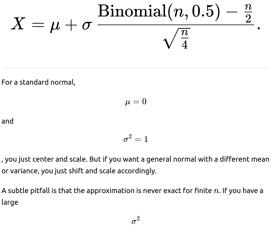
Approximate Approach Using the Central Limit Theorem
Another (simpler but approximate) method is to sum a large number of independent Bernoulli draws:

Python Pseudocode for Box-Muller with a Bernoulli Generator
Below is an illustrative Python code snippet for a basic approach. It shows how you might go from a Bernoulli generator to a uniform in [0,1), then transform that into a standard normal variable with Box-Muller.
import math
import random

def bernoulli_generator(p=0.5):
    """
    Returns 0 with probability (1-p) and 1 with probability p.
    """
    # In a real scenario, you might read from specialized hardware or
    # a lower-level random bit generator. For demonstration, we use random.random()
    # but pretend it's calling a Bernoulli(p).
    return 1 if random.random() < p else 0

def generate_uniform_from_bernoulli(num_bits=32):
    """
    Generate a float in [0,1) by collecting num_bits from the bernoulli_generator.
    """
    result = 0
    for i in range(num_bits):
        bit = bernoulli_generator(0.5)  # fair coin
        result = (result * 2) + bit
    # divide by 2^num_bits to shift into [0,1)
    return result / (2 ** num_bits)

def box_muller_from_bernoulli():
    # 1) Generate two Uniform(0,1)
    u1 = generate_uniform_from_bernoulli(num_bits=32)
    u2 = generate_uniform_from_bernoulli(num_bits=32)

    # 2) Apply the Box-Muller transform
    z1 = math.sqrt(-2.0 * math.log(u1)) * math.cos(2.0 * math.pi * u2)
    # z2 = math.sqrt(-2.0 * math.log(u1)) * math.sin(2.0 * math.pi * u2) # If you need another sample

    return z1

# Example usage
samples = [box_muller_from_bernoulli() for _ in range(10000)]
# 'samples' should now contain ~10,000 draws from a standard normal distribution
In production, you could refine this for performance and precision (e.g. using a different number of bits for the fractional part, or using the Marsaglia polar method which often is faster).
Potential Follow-up Interview Questions
Below are typical deeper questions an interviewer at a top tech company might ask, along with detailed answers and potential pitfalls.
How do you ensure that the Bernoulli generator is unbiased if p≠0.5?
You can use a standard “von Neumann extractor” technique to turn a biased coin into an unbiased coin, with some caveats regarding efficiency:

Provided each pair is i.i.d. from Bernoulli(p), the probability of (1,0) is the same as (0,1), namely p(1−p). This approach outputs a fair bit. However, you may have to discard many pairs in the worst case, hurting efficiency if p is very close to 0 or 1. Once you can generate unbiased bits, you can proceed with the same pipeline (generate uniform, then apply Box-Muller).
Pitfall: If you do not address a biased coin, your final normal distribution will be skewed or will not have the correct variance.
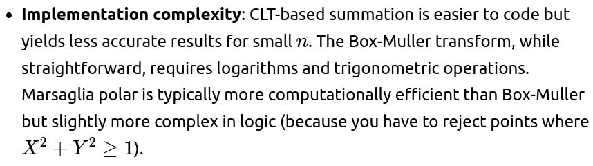
Why use the Box-Muller transform versus the Central Limit Theorem approach?
Exactness: The Box-Muller and Marsaglia polar methods produce exact draws from N(0,1) when fed truly uniform (0,1) samples. The CLT-based approach is only an approximation for finite n.

Performance: The sum-of-Bernoullis approach might be quite slow if you need a large n to ensure a good normal approximation. Box-Muller or Marsaglia only needs a small fixed number of bits to achieve each sample.
Pitfall: People sometimes assume the CLT approach is “good enough” for any n. In certain high-precision or tail-heavy use cases, you might need a fairly large n to approximate the normal distribution in the tails accurately.

Could we do inverse transform sampling from the normal’s CDF using Bernoulli bits?
While theoretically possible, the inverse transform method for the normal distribution involves the error function (erf) as part of the inverse CDF. Numerically computing the inverse error function to high precision can be expensive. You would still need uniform samples in (0,1) anyway. Hence, methods like Box-Muller or Marsaglia polar are usually simpler.
Pitfall: Some might try to directly approximate the normal CDF’s inverse with polynomial or rational approximations. It can be done, but it’s not necessarily more efficient or simpler than Box-Muller or Marsaglia.
How would you generate a truncated normal from a Bernoulli generator?

Pitfall: If you’re dealing with a very narrow truncation interval deep in a tail, you might have to do many rejections, so specialized sampling methods (e.g., truncated normal sampling via accept-reject bounding or tailored transformations) can be more efficient.
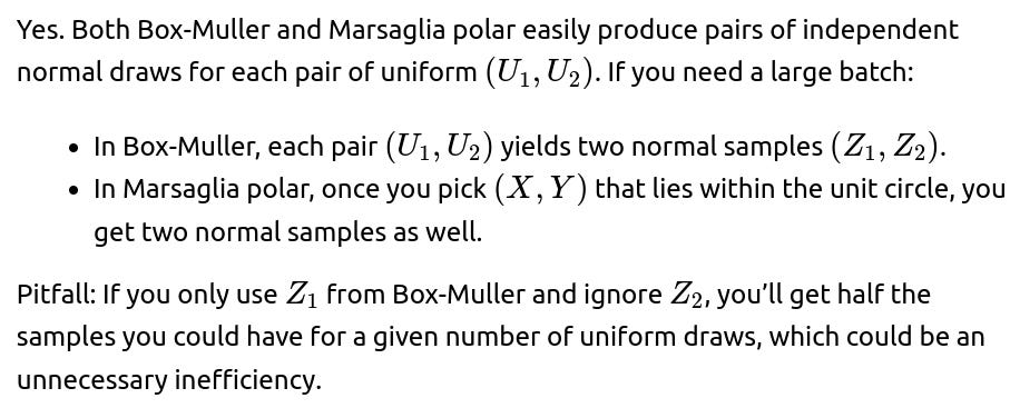
Does the method scale if we need multiple i.i.d. standard normal draws in a single step?
What if precision is limited and we cannot generate as many bits as we want?
If the Bernoulli generator or the system you run on has limited precision (for instance, if you only can easily get 16 bits at a time):
You can still concatenate multiple calls to get more bits, but you might do it more carefully to avoid floating-point issues.
If you are severely constrained in bits, acceptance-rejection or approximate table-based sampling might be more suitable.
Pitfall: Relying on too few bits can cause subtle biases in the tails of the normal distribution where very small or very large values rely on extremely rare uniform draws.
Could you do rejection sampling without generating Uniform(0,1)?
Yes. You can do acceptance-rejection sampling directly using Bernoulli bits, but typically you’d still be implicitly forming some uniform threshold. For example, the Marsaglia polar approach (where you accept or reject points in the unit disk) can be seen as a purely Bernoulli-based scheme if you cleverly interpret your random bits in 2D. However, conceptually it’s simpler to think of it as generating uniform [0,1] or [−1,1] variables.
Pitfall: If you skip the uniform generation step or do not track your threshold carefully, it’s easy to design a flawed acceptance-rejection scheme that biases the samples.
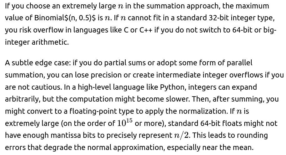
Could the sum-of-Bernoullis approach cause any overflow if n is huge?
If n is so large that storing Binomial(n,0.5) is not feasible in standard integer types, you might need big-integer data structures or you might break the sum into chunks. For practical ranges of n, it’s often safe in a 64-bit integer, but in some extremely large n scenarios, you have to be cautious.
Pitfall: Failing to handle large integer sums leads to integer overflow, destroying the distribution’s correctness and leading to silent, incorrect results.
Are there any big performance differences between Box-Muller and the Marsaglia polar method?

How would you confirm empirically that the generated samples are truly standard normal?
You can apply standard statistical tests:
Histogram: Compare the histogram of generated samples to the theoretical bell curve.
Q-Q Plot: Plot the quantiles of the generated samples against the quantiles of the standard normal distribution. If the samples are truly normal, the points will lie close to the diagonal.
Statistical Tests: Use tests such as the Kolmogorov-Smirnov test, the Anderson-Darling test, or the Shapiro-Wilk test to check normality.
Mean and variance: Check if the sample mean and variance are close to 0 and 1, respectively.
Pitfall: A single test or small sample might be misleading, especially in the tails. Testing thoroughly with large sample sizes is advisable for high confidence.
What if the interviewer asks about potential non-uniformities from floating-point rounding?
When forming a fraction from bits, you do have to consider floating-point representation carefully. In practice:
If you accumulate bits as an integer and then do a division by ParseError: KaTeX parse error: Expected 'EOF', got '_' at position 13: 2^{\text{num_̲bits}} in floating-point, you can represent each fraction exactly for up to 53 bits in double precision (the 53-bit significand in a 64-bit double can represent powers of two exactly).

Pitfall: If you try to use, say, 60 bits to create a fraction in standard double precision, the fraction might not be exact. This might create extremely subtle biases or missing representable intervals. In many real-world applications, 32 to 53 bits of precision is adequate.
How do you generate a normal random variable if the Bernoulli generator is extremely slow?
In some hardware or simulation contexts, calling the Bernoulli generator might have a high latency. To mitigate:
You can “batch” multiple bits at once, or buffer them, so you only occasionally call the underlying generator.
You can also choose an algorithm that’s more bit-efficient. For instance, some advanced methods might do partial acceptance to reduce the expected number of bits needed for each sample.
Pitfall: Overusing or discarding bits might waste valuable randomness. This can degrade performance if each bit is expensive.
Could quantum or hardware-based random number generators change the approach?
If you have a hardware random number generator that’s truly uniform in [0,1) or that can directly output floating-point random samples, you might bypass all this bit manipulation and directly use library-based normal generation routines. But if all you have is a physical device that flips biased coins, you can still implement the same logic. The mathematics remains identical.
Pitfall: Over-reliance on hardware devices for large-scale sampling might require calibration, speed considerations, or potential correlations if the device has drift or non-idealities over time.
Summary of Key Points
You can convert a Bernoulli generator into a uniform [0,1] generator by gathering enough bits into a binary fraction.
Using that uniform generator, you can create standard normal samples via the Box-Muller transform, the Marsaglia polar method, or inverse transform sampling.
If you need an approximate normal quickly, you can sum a large number of Bernoulli(0.5) draws and standardize the result, though it’s only exact in the limit of large n.
Make sure the Bernoulli bits are unbiased, or correct them if they’re not.
Beware of corner-case numerical issues: U=0 in Box-Muller, large n in CLT, or floating-point precision limits.
Test the resulting samples via histograms, Q-Q plots, or formal normality tests to confirm correctness.
Below are additional follow-up questions
How would you handle parallelization or concurrency when generating standard normal samples from a Bernoulli generator?
One potential scenario is running the sampling algorithm on multiple threads or multiple machines simultaneously. If each process or thread uses the same Bernoulli generator (or a shared state), care must be taken to avoid race conditions and to ensure independent random streams:
When multiple threads call the Bernoulli generator concurrently, you need a thread-safe mechanism to produce random bits. Otherwise, two threads might read or write overlapping states, resulting in correlated or duplicated bits. One common solution is to use independent seeds for each thread, effectively creating separate streams of bits that do not overlap.
A subtle edge case is if you rely on shared global counters or buffers of bits. An uncoordinated refill of the buffer can cause concurrency bugs, leading to repeated sequences of bits in multiple threads. This can severely degrade the statistical properties of your normal samples. Proper synchronization (e.g., with locks or lock-free data structures designed for concurrency) or separate dedicated Bernoulli sources for each thread is essential.
In a high-performance computing environment with thousands of cores, each node or thread is often given a unique seed and offset in the random stream. For instance, you might use a known technique like “skip-ahead” in pseudo-random number generation. But with a hardware Bernoulli generator, you must ensure each thread receives a properly partitioned share of bits. Failing to do so can introduce subtle correlations or repeated sampling sequences that are extremely difficult to detect unless you perform extensive statistical tests.
If each thread or machine uses a different method (e.g., one uses Box-Muller, another uses Marsaglia polar) or partial sums, you must ensure they all produce high-quality normal samples. The method used can differ as long as the seeds and streams are truly independent. But if you try to feed the same bits into different transformations, you might get correlated outputs, so that typically is best avoided unless carefully planned.
How do you handle cryptographic security requirements when generating normal samples?
If your application is security-sensitive—e.g., generating noise for a cryptographic system—you might need cryptographically secure random variables. A naive Bernoulli generator, if not based on a cryptographically secure source of bits, could allow adversaries to predict future samples, compromising the security of your system.
In such a setting, you would employ a secure hardware random number generator or a cryptographically secure pseudo-random number generator (CSPRNG). The Bernoulli bits must be unpredictable. Then you can feed these bits into your normal sampling routine (Box-Muller, Marsaglia, etc.). The next subtlety: to maintain security, you must ensure no side-channels can leak the bits or partial information about the generated samples. Side-channel attacks might exploit timing differences in your acceptance-rejection steps or repeated calls to expensive math functions.
In cryptographic settings, you must also worry about the distribution’s exactness. If your normal sampling is used in a zero-knowledge proof or advanced crypto protocol, small statistical deviations can be exploited. High-precision or advanced sampling methods with proven bounds on distribution correctness may be required. An approximate approach like summing Bernoullis (CLT) might not be acceptable because it introduces distributional errors that an adversary could exploit.
Can the Bernoulli generator’s output be correlated over time, and what happens if so?
A typical assumption is that each bit from the Bernoulli generator is i.i.d. with probability 0.5 for heads or tails. However, in some real-world hardware or software implementations, especially low-quality or incorrectly seeded generators, bits might show correlations. For example, the chance of a bit being 1 could depend on the previous bit.
Correlations destroy the assumption of independence, which underpins uniform (0,1) generation. Consequently, your derived normal samples might be biased or correlated. You could see non-Gaussian behavior, especially in tail events. For instance, certain patterns might appear more often than they should.
If correlation is suspected, rigorous statistical tests (like autocorrelation tests, runs tests, or the NIST test suite for randomness) can help detect patterns. If correlation is found, you might attempt to decorrelate the stream via re-seeding or advanced post-processing (like hashing blocks of bits). But advanced post-processing can add overhead and may still not fully repair a severely correlated bit source.
How might you generate a correlated multivariate normal distribution if you only have a Bernoulli generator?
A multivariate normal can be constructed by first generating multiple independent standard normals, then applying a linear transformation that induces the desired covariance. The steps are:
Generate a vector of independent standard normals


Potential pitfalls include numerical instability or ill-conditioned covariance matrices (where the matrix is nearly singular). In these cases, computing the Cholesky factor can fail or lose precision, resulting in inaccurate correlation. Also, if the Bernoulli generator is correlated or not truly uniform, the final correlation structure in
Furthermore, the dimensionality matters. Generating large dimensional correlated normals might require significant random bits. Each dimension needs multiple calls to the Bernoulli generator, so you can quickly run into performance bottlenecks.
What if you have strict memory constraints and can only store a small buffer of bits at a time?
Memory constraints can arise in embedded systems or very resource-limited devices. Storing, say, 1 MB of random bits at once might be impossible. Instead, you can generate bits on-the-fly:
Generate a small batch of Bernoulli bits.
Convert them to one or more uniform (0,1) samples.
Apply your normal transform (e.g., Box-Muller).
Discard or reuse leftover bits if any remain, then get more bits as needed.
A tricky edge case arises when your method demands a variable number of bits, such as with rejection sampling (Marsaglia polar) where you might reject many pairs of (X,Y). You could run out of bits mid-computation. You must carefully design a pipeline that gracefully requests new bits without partially discarding a half-computed sample.
If you are extremely memory-limited and must store partial results for the next iteration, you risk states or partial sums that can cause subtle sampling biases if not handled correctly. Testing is essential to ensure that your bit usage and partial remainders do not accumulate rounding or indexing errors.
How do you handle generating normal variables on GPUs or specialized hardware accelerators with only Bernoulli-like random sources?
Modern GPUs often have built-in hardware instructions for generating uniform random numbers, but if you only have a Bernoulli source, you can still adapt the methods:
You would collect bits in parallel across many GPU threads. Each thread (or warp) can then assemble a fraction in [0,1), apply the Box-Muller transform, and produce a normal sample. The challenge is ensuring each thread gets unique, uncorrelated bits. One approach:
Assign each thread a unique index.
Use that index, combined with a global seed, to generate a distinct offset in the Bernoulli sequence so each thread sees a different chunk of bits.
Alternatively, if you have a hardware random function that outputs single bits, each thread can read from an atomic or locked queue of bits. But that might significantly degrade performance due to contention.
Pitfalls in GPU environments include warp divergence (e.g., if you rely on acceptance-rejection, some threads might reject more often and cause branches in the code). You also risk partial usage of bits if the threads that accept or reject at different rates cause out-of-sync consumption of the shared bit buffer. This must be carefully managed, often with an approach that re-synchronizes or uses local caching of bits.
If you only have limited precision floating-point (e.g., half-precision), does that affect generating normal samples?
In half-precision (16-bit floating point), you have fewer bits of mantissa, so your uniform sampling in [0,1) might not be able to represent fine increments. For something like Box-Muller, near zero values of

could become underflow, and the logarithm might produce inaccurate or infinite results. This can distort the tail distribution of the normal.
You might mitigate this by generating and performing initial calculations in higher precision (e.g., integer or 32-bit float) before converting to 16-bit. If your environment only supports half-precision in hardware, you must handle certain expansions in software. This can slow your method down but ensure correctness. The key pitfall is losing the accuracy needed to produce correct tails, which can matter in some applications (e.g., modeling extreme events in finance or engineering).
How can you detect if your normal generator from Bernoulli bits drifts from the standard normal over time?
Drift can occur if the Bernoulli source slowly changes its bias due to temperature, hardware aging, or software bugs that build up. To detect drift, you could:
Continuously or periodically test newly generated samples using rolling statistical tests. For instance, maintain an online estimate of mean and variance, then check if they deviate significantly from 0 and 1, respectively.
Perform a specialized normality test (e.g., Shapiro-Wilk) in a rolling or batched manner on the recent sample set.
Look at the tails specifically. Track how frequently you see samples beyond 3 standard deviations or 5 standard deviations, comparing that rate to the theoretical N(0,1) expectation.
A subtle scenario is if the Bernoulli generator becomes systematically biased, say drifting from 0.5 to 0.5001. This might not strongly affect the mean or variance in the immediate term, but it can accumulate a subtle difference in tail probabilities. Comprehensive tests or calibration can catch such slow drifts over time.
If you need a log-normal distribution instead of a normal one, how do you proceed?


What strategies might you use if you only need “roughly” normal noise, and you want to minimize calls to the Bernoulli generator?
In some applications (e.g., simulations or quick heuristics) you may only need a shape that loosely resembles a Gaussian, not an exact distribution. You can reduce calls to the Bernoulli source in several ways:
Use a small random seed from the Bernoulli generator once, then expand that seed into many pseudo-random uniform samples in software (like using an Mersenne Twister or an Xorshift algorithm). This drastically cuts down on hardware calls. You lose perfect hardware randomness but for some engineering tasks, that might be acceptable.
Use a Ziggurat algorithm or other sampling methods known to be bit-efficient.
Use an approximation method such as piecewise linear approximation of the normal CDF. You only need a handful of random bits to select which piece you fall into. This method may be less accurate in the tails but can be extremely fast.
The main pitfall is that any pseudo-random approach or approximate piecewise method might exhibit small biases. Over large runs, these biases can become significant if your application is sensitive to exact tail probabilities or distribution shape. Also, ensuring good seeding and no accidental correlations is essential.
Could you use a deterministic (non-random) approach such as quasi-Monte Carlo to approximate normal sampling from Bernoulli bits?
Quasi-Monte Carlo (QMC) methods use low-discrepancy sequences instead of purely random draws. They typically yield faster convergence in numerical integration tasks. However, if you specifically need random normal samples (e.g., in a stochastic simulation or randomized algorithm that relies on true randomness), QMC might not be appropriate. QMC effectively removes randomness in favor of deterministic coverage of the domain.
Even if you wanted to emulate QMC, you’d still need a sequence of bits to guide the generation of these low-discrepancy points. If your Bernoulli generator is truly random, you lose the main advantage of QMC’s deterministic structure. QMC has also been adapted to produce “quasi-Gaussian” samples by transforming a low-discrepancy sequence, but it’s not truly random.
A pitfall arises if you mix partial random bits with a low-discrepancy sequence incorrectly, leading to a confusing distribution that’s neither purely random nor fully deterministic. That can yield unpredictable results in a modeling or simulation context.
Are there scenarios where we should avoid the Box-Muller or Marsaglia polar approach altogether?
Box-Muller and Marsaglia polar are great general-purpose methods. However, there are scenarios where specialized sampling methods might be better:
Truncated normals with tight bounds: Repeated rejection in Box-Muller or Marsaglia may be very inefficient. Specialized truncated normal samplers can be far more efficient.
High-precision tail modeling: Some advanced acceptance-rejection methods or sampling methods designed with a stable approach to extreme tails may be superior if your application is extremely sensitive to rare events.
Discrete approximations: In extreme embedded contexts with minimal hardware floating-point capabilities, summing Bernoullis might actually be simpler than implementing logs or trig functions.
Pitfalls occur if you reflexively apply Box-Muller in a scenario where repeated rejections or expensive function calls hamper performance or create numerical issues.
How do you ensure reproducibility in your normal sample generation when you have a Bernoulli source?
Reproducibility typically means that each run of your program or experiment yields the same sequence of random numbers if started with the same seed. If your Bernoulli generator is hardware-based and truly random, it might not be reproducible in the strict sense. In research or debugging contexts, you may want to store the entire sequence of bits or store the seed to a pseudo-random Bernoulli generator, so you can replay it.
If you want reproducible results but only have a hardware-based Bernoulli generator, you can:
Collect enough bits once, store them in a file. Future runs read from that file, guaranteeing the same sequence.
Seed a pseudo-random generator with a known seed, then produce Bernoulli bits in software. This is the usual approach in simulations and unit tests.
A subtle pitfall is that floating-point differences across hardware (e.g., GPU vs. CPU, or different CPU architectures) can cause small divergences in the final normal values, even if the bit streams match. This might matter if you require bitwise identical results across platforms. In such a scenario, ensure the exact same math libraries and rounding modes are used or consider an integer-based or rational-based method.
How would you handle validation in a regulated industry, like medical devices or finance, where normal sampling must meet strict standards?
Regulated industries often require documented evidence that the random number generation meets certain statistical properties. You might need to:
Provide a formal proof or extensive test results (e.g., running millions of samples through the Dieharder, TestU01, or NIST suites).
Have a traceable calibration procedure for your hardware Bernoulli generator (if it’s a physical device).
Document your transformations (Box-Muller, Marsaglia, or other) with references to known statistical correctness.
Ensure version control and full reproducibility for audits.
One pitfall is that certain regulators might demand that you demonstrate your system’s behavior under worst-case conditions—such as partial hardware failures or temperature extremes that bias your Bernoulli generator. If you cannot show that these conditions do not adversely affect your normal sampling (e.g., produce incorrect tail probabilities), you might fail a regulatory audit.
How can floating-point rounding in the logarithm or division steps for the Box-Muller or Marsaglia method lead to biases?

is extremely small, the logarithm might be large but truncated in floating point. This can cause “binning” in the distribution, especially in the extreme tails.

is extremely close to 0. This might cause certain tail values to appear with slightly incorrect probabilities.
The subtle pitfall is that typical tests of normality may not easily catch such small floating-point biases if they only focus on the central region. However, in tail-sensitive applications (like risk management or certain scientific computations), those tail inaccuracies can matter. Solutions include using double precision or higher-precision libraries for the critical steps, or adding checks that clamp values to safe ranges.
How does the Ziggurat algorithm compare when using a Bernoulli generator?
The Ziggurat algorithm is another fast method for generating normal random variables. It relies on piecewise regions (often rectangles plus one tail region) and acceptance-rejection. Typically, it is described in terms of uniform random draws in [0,1). You could implement it with a Bernoulli generator by first generating a uniform random float. The rest of the steps remain the same, partitioning the normal distribution into “steps” or rectangles.
A possible challenge is that the Ziggurat algorithm usually stores precomputed tables for boundaries. If you have limited memory, that table might be large for improved precision. Another pitfall is that if your uniform generation is not truly uniform (e.g., correlated bits or partial biases), you can cause subtle artifacts in the distribution shape. Nonetheless, if done carefully, Ziggurat can be more efficient than Box-Muller or Marsaglia in many scenarios.
How might summation-based approaches be generalized to produce normal distributions with different means or variances?


so the scaled binomial captures enough tail. Otherwise, the resulting distribution might not have the correct shape in the far tails. This can lead to underestimation or overestimation of extreme events.
How could underflow or overflow occur when summing a large number of Bernoulli bits?

How might partial usage of bits in acceptance-rejection schemes lead to subtle bias?
Some acceptance-rejection methods, like the Marsaglia polar method, require checking a condition (e.g.,

). You might have generated X and Y from bits that form uniform (−1,1). If S≥1, you discard X and Y. But you might still have leftover bits that you partially read and used to form X or Y. If you improperly recycle those bits or fail to properly discard them, you introduce correlation or reuse partial randomness in the next iteration. That leads to biased sampling.
A related pitfall is if your code tries to “optimize” by reusing the bits that were not fully consumed in the partial generation of X or Y. For instance, if you form X from 10 bits, Y from 10 bits, but you read them from a 32-bit chunk, you have 12 leftover bits. If you keep reusing these bits incorrectly for the next iteration, you might inadvertently tie the next sample to the prior sample’s partial bits. A safe approach is typically to use a well-defined chunk size for each sample. Any partial chunk is either carefully tracked or entirely discarded.
How do you ensure that your random normal samples remain stable over different compiler optimizations or hardware instructions?
Modern compilers can optimize floating-point operations differently (e.g., using FMA instructions, rearranging sums, or employing approximate trig/log instructions). This can alter the exact numeric rounding and produce small changes in your normal draws. If stability is essential (for reproducibility or regression testing), you can:
Force specific compiler flags that disable certain floating-point optimizations (like -ffp-model=strict in some compilers).
Use a well-tested math library that guarantees bitwise reproducibility for log, sin, cos, etc.
Store intermediate steps in double precision or higher to reduce rounding differences across platforms.
A subtle pitfall is that some HPC or GPU libraries have faster but approximate math implementations for exp, log, sin, etc. This can shift the distribution slightly, particularly in the tails. These differences might or might not matter for your application, but they can show up in QA or sensitive scientific simulations.
How would you adapt these methods if the Bernoulli generator has a high latency but can deliver a large block of bits in a single operation?
If the Bernoulli generator is slow but can provide big blocks of bits occasionally, a strategy is to buffer those bits:
Request a large block of bits from the generator.
Store them in a local buffer in memory.
Draw from the buffer to generate uniform (0,1) samples, then normal samples, as needed.
When the buffer is depleted, request another large block.
Pitfalls arise if the buffer approach is implemented incorrectly—for example, partially reading from the buffer could overlap or skip certain bits. Another pitfall is if the system is event-driven and you do not realize that the block might take time to arrive, so you inadvertently create idle wait times or concurrency issues. Proper double-buffering (where you request a new block before you run out of the current one) can keep your pipeline fed consistently.
How would you debug or diagnose subtle biases in your normal sampling that might only appear in large-scale runs?
Diagnosing subtle biases in normal sampling often requires large sample sizes, because typical tests (like Q-Q plots or standard normality tests) may appear fine for modest sample sizes. Techniques:
Collect tens of millions (or more) of normal samples and run heavy-duty test suites (e.g., TestU01’s BigCrush).
Look at distribution tails explicitly, e.g., how often samples exceed 4 or 5 standard deviations. Compare that to the theoretical normal tail probability. If you see a significant deviation from the expected rate, suspect a bias in bit usage or a small correlation in your Bernoulli source.
Compare your normal-sample statistics across multiple seeds or multiple hardware states. If biases appear only for certain seeds or at certain times, you might suspect a concurrency or seed management issue.
Deploy incremental checks in production if feasible. For example, if your system is used daily, log a random subset of generated samples. Over weeks or months, analyze them offline to see if there is a drift or systematic deviation from normal.
A big pitfall is failing to test thoroughly in the tails, where small errors can matter greatly. Another pitfall is mixing your production usage with your test usage in a way that seeds or concurrency differ, so your test scenario does not replicate real conditions. You must replicate real usage patterns as closely as possible to detect real-world biases.