
ML Interview Q Series: Geometric Distribution for Time Until Biased and Fair Coins Match

Browse all the Probability Interview Questions here.
You toss a biased coin with probability p of heads, while your friend tosses at the same time a fair coin. What is the probability distribution of the number of tosses until both coins simultaneously show the same outcome?
Short Compact solution
By conditioning on whether the biased coin lands heads or tails, we see that the probability of getting the same result (both heads or both tails) on a single toss is (1/2)p + (1/2)(1−p) = 1/2. Therefore, the number of tosses until the first time both coins match follows a geometric distribution with parameter 1/2, leading to an expected value of 2 and standard deviation sqrt(2).
Comprehensive Explanation
The probability of a match on a single toss
We have two coins:
Coin A: Biased, with probability p of landing heads.
Coin B: Fair, with probability 1/2 of landing heads (and 1/2 of landing tails).
To match on a single toss, either both coins show heads or both show tails. The probability of both showing heads is p * (1/2). The probability of both showing tails is (1−p) * (1/2). Adding these probabilities gives:
p*(1/2) + (1−p)*(1/2) = (1/2)p + (1/2)(1−p) = 1/2.
Hence, on any given toss, the probability of a “match” is 1/2, regardless of p.
Geometric distribution of the number of tosses
We define a random variable X to be the number of tosses needed until the first match occurs. Since each toss is independent and has a success probability of 1/2 (i.e., a match), X follows a geometric distribution with parameter r = 1/2. That means:
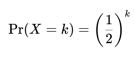
for k = 1, 2, 3, ... if we use the version of the geometric distribution where the probability mass function is (1−r)^(k−1) * r. Because r = 1/2, (1−r) = 1/2, so (1−r)^(k−1)r = (1/2)^(k−1)(1/2) = (1/2)^k.
Expected value and standard deviation
For a geometric random variable X with parameter r, the expected value E[X] = 1/r, and its standard deviation SD[X] is sqrt((1−r)/r^2). In our case r = 1/2, so:

Why conditioning works here
An alternative explanation is to note that if we are waiting for both coins to match, we can think of each trial as a “success” if they match and a “failure” otherwise. Because each toss is independent, and the probability of success (match) on any single toss is 1/2, the time to the first success is governed by the geometric distribution with parameter 1/2.
Potential Follow-up Questions and Detailed Answers
What if the coin tossed by the friend were also biased with probability q of heads?
If both coins are biased—coin A has probability p of heads and coin B has probability q of heads—then the probability of a match on a single toss is:
pq + (1−p)(1−q).
In that situation, the probability of success (match) on any given toss is pq + (1−p)(1−q). Thus, the number of tosses until the first time the two coins show the same outcome is still geometric, but the parameter becomes r = pq + (1−p)(1−q). One can then compute the expected value as 1/r and the standard deviation as sqrt((1−r)/r^2). In more detail:
Probability of both heads: p*q
Probability of both tails: (1−p)*(1−q)
Hence the match probability is pq + (1−p)(1−q). This sum can be simplified to pq + 1 − p − q + pq = 2pq + 1 − p − q, but the form pq + (1−p)*(1−q) is often clearer for conceptual understanding.
How does one implement a simulation in Python to verify this result?
We can simulate multiple independent experiments, each consisting of repeated tosses until the first match occurs. We then observe how many tosses it takes on average and check how closely the empirical distribution aligns with the theoretical geometric distribution. A simple Python code snippet for this might be:
import random
import statistics

def simulate_geometric(p, num_trials=10_000_00):
    # p is the probability of match in a single toss
    results = []
    for _ in range(num_trials):
        count = 0
        while True:
            count += 1
            # We "succeed" with probability p
            if random.random() < p:
                results.append(count)
                break
    return statistics.mean(results), statistics.pstdev(results)

# For the scenario in the question, p = 0.5
mean_estimate, std_estimate = simulate_geometric(0.5)
print("Estimated mean:", mean_estimate)
print("Estimated standard deviation:", std_estimate)
In practice, the estimated mean should be close to 2, and the estimated standard deviation close to sqrt(2), as the number of trials grows large.
Is there a scenario where the geometric distribution would not apply?
The geometric distribution assumption relies on the key property that each toss is an independent Bernoulli trial (with the same probability of success each time). If there were any dependency from one toss to another (for example, if the probability p changed over time or if the outcome of the second coin depended on the first coin’s history), the number of tosses until the first match might not be geometric. The geometric distribution applies precisely because each pair of tosses is independent and identically distributed, and the probability of a match remains constant at every trial.
Could the result differ if we used the “shifted” version of the geometric distribution?
There are two common definitions of a geometric random variable:
Definition A (most common in probability texts): X counts the number of Bernoulli trials up to and including the first success (so X = 1, 2, 3, …).
Definition B: X counts the number of failures before the first success (so X = 0, 1, 2, …).
In either definition, the essential shape of the distribution is the same, but the support and the exact pmf formula differ by 1 in the indexing. In our question, we explicitly define X as “the number of tosses until the coins first match,” implying the first definition (we start counting at 1, and we stop the moment we see the first match). Consequently, the pmf is (1−r)^(k−1)*r for k ≥ 1. If we used the second definition, we would have X counting the number of non-matching tosses before the first match, but the underlying probability structure is still the same. It is simply a matter of how we index X.
What if p = 0 (or p = 1)? Does the formula still hold?
If p = 0, coin A always lands tails, while coin B is fair. The probability of a match is the probability that coin B also lands tails, which is 1/2. The distribution of the number of tosses until the first simultaneous tail–tail remains geometric with parameter 1/2.
If p = 1, coin A always lands heads, while coin B is fair. The probability of a match is then the probability that coin B also lands heads, again 1/2. So even in these extreme cases, the parameter is 1/2, and the geometric distribution outcome remains valid.
Thus, the result is robust even at the boundary values of p.
How can we interpret this result intuitively?
An intuitive explanation is: The friend’s fair coin is equally likely to match or mismatch whatever outcome the biased coin shows. Regardless of the biased coin’s probability p, in every toss the fair coin yields heads or tails with probability 1/2 each, so it “lines up” or “does not line up” with the biased coin half of the time on average. Consequently, it takes on average 2 tosses to get a match, which is exactly what we find from the geometric distribution with parameter 1/2.
All these points emphasize that the core reason the number of tosses follows a geometric distribution with parameter 1/2 is that each trial’s success (matching) occurs independently with probability 1/2, no matter what p might be.
Below are additional follow-up questions
What if we only partially observe the outcomes of each toss?
One interesting variant arises if we do not fully observe both coins on every toss. For instance, suppose we only see whether at least one coin landed heads, but we do not know exactly which coin (or coins) produced the head. This partial observability makes it impossible to directly know if a match has occurred on any particular toss. Consequently, we cannot simply use “match vs. no match” as a Bernoulli trial with probability 1/2 each time. Instead, we would have a more complicated hidden-state scenario:
State 1: Coins match.
State 2: Coins do not match.
But we only observe some noisy signal (e.g., “there is at least one head”). In such a situation, the time until we infer that a match has happened might be significantly different from the geometric distribution time, because partial observations prevent us from directly detecting the exact event we care about. This scenario is reminiscent of Hidden Markov Models (HMMs), where the underlying process (matching vs. not matching) is hidden, and we see incomplete evidence of outcomes. We would have to do Bayesian updates to maintain beliefs about whether a match has occurred, which could lead to a more complex distribution for the stopping time.
Key pitfall or edge case:
We cannot treat each trial as a simple Bernoulli(1/2) event because we do not have direct visibility into the event of interest. Consequently, the well-known closed-form results for the geometric distribution no longer apply without additional modeling steps.
How does the distribution change if the biased coin’s probability p is itself random?
Another subtle variant is when the biased coin’s probability of landing heads, p, is itself drawn from some distribution (for instance, a Beta distribution) and does not remain fixed across trials, but rather is an unknown random quantity from the start. This leads to a “compound” or “mixed” model. Specifically:
Before the first toss, p is drawn from some prior distribution, say Beta(α, β).
We then repeatedly toss the coin under that random p, while your friend tosses a fair coin.
We want the distribution of the time until the two coins match. Because p is random, the match probability on each trial is no longer a fixed 1/2. Instead, on each trial, it will be (1/2)p + (1/2)(1−p), but p is itself a latent random variable. The unconditional probability of a match on a single trial is then the expected value (with respect to p) of (1/2)p + (1/2)(1−p). One can show this still simplifies to 1/2 when we look at the unconditional probability, but the subtlety is that if after each trial you update your knowledge of p (for instance, in a Bayesian inference setting), the match probability for subsequent tosses might shift. If p is truly fixed but unknown, repeated observation of heads or tails on coin A would give partial information about p, and we might do real-time updates. However, for the simpler scenario where p is not updated by observation (i.e., we treat p as a fixed but unknown constant from the standpoint of the coin’s actual process), the unconditional match probability remains 1/2 each toss, so we still get a geometric distribution. But if we condition on the observed flips to update our knowledge of p, we might no longer treat each toss as i.i.d. from the perspective of the observer.
Key takeaway:
From the coin’s intrinsic point of view, if p is drawn once and remains fixed, each toss still has the same match probability of 1/2, so the time until a match is geometrically distributed with parameter 1/2.
From the observer’s point of view, if learning or Bayesian updating is happening, the observer’s belief in p changes, which can add complexity to how we interpret or detect the match event over time.
What if there is a small chance that the coin lands on its edge?
Sometimes real physical coins can land on their edge (albeit with very small probability). Denote that probability by ε. Then each toss has three possible outcomes: heads, tails, or edge. If we define “match” strictly as “both show the same face (heads or tails), ignoring edges,” we have to consider how the edge outcome complicates the process:
With probability ε for coin A and 1/2 for coin B, or vice versa, or both landing on edges, the result might not count as heads or tails for either coin, thus not leading to a “match” or “mismatch” in the usual sense. This effectively introduces “no event” tosses in which we neither succeed nor fail but must toss again.
One way to handle this is to treat the occurrence of an edge as a “retry” event that does not change the system state. If both coins have a probability ε of landing on the edge, the probability that neither coin lands on the edge is (1−ε)*(1−ε). Condition on that to see the probability of heads/tails match:
If no edge occurs, then the chance they match (both heads or both tails) within that subspace is still 1/2.
But each trial only has a (1−ε)^2 chance of producing a valid heads/tails pair at all.
Hence, effectively we only get a “valid toss” with probability (1−ε)^2, within which the match happens with conditional probability 1/2. From the perspective of counting only valid tosses, the distribution is still geometric with parameter 1/2. However, from the perspective of counting every attempt (including edges), the number of attempts to see a valid match is geometrically distributed with a success probability (1−ε)^2 * (1/2). Because many tosses might be wasted landing on edges, the expected time until a match can become quite large if ε is not negligible.
Pitfall:
Real coins do not have exactly zero probability of landing on edges, so in extremely precise physical modeling or extremely large sample sizes, this tiny probability might introduce more complicated behavior. For most practical purposes (ε near 0), the simpler model suffices.
What if we change the problem to require that both coins match in a specific way (e.g., both heads) before stopping?
Instead of stopping at the first time both coins show the same outcome (heads–heads or tails–tails), suppose we only stop when they both land heads. Now, the probability of that specific event (heads–heads) in any single toss is p*(1/2). This is smaller than 1/2 (unless p = 1). Therefore, the number of tosses until the first time both show heads is still geometrically distributed, but now with parameter p*(1/2). In other words:
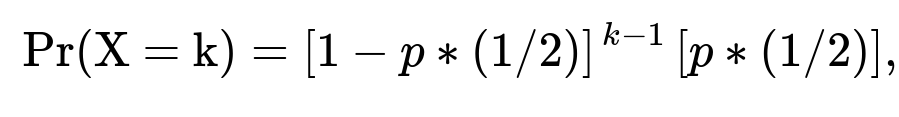
where X is the number of tosses to see the first heads–heads. Its expected value would be 1 / (p*(1/2)) = 2 / p. So the mismatch probability (or “failure” probability) each round is 1 − p/2, which includes any scenario that is not heads–heads (i.e., the second coin is tails, or the first coin is tails, or both are tails).
Pitfall:
The candidate might assume incorrectly that the event “both heads” still has probability 1/2. That confusion arises from the original scenario where “match” included both heads–heads and tails–tails. Changing the success criterion to only heads–heads definitely changes the success parameter and therefore the distribution’s shape.
What if we need to observe multiple consecutive matches before stopping?
Instead of stopping as soon as we see a single match, we might require two (or more) consecutive matches (e.g., we need match on toss t and match on toss t+1 for the process to stop). In that scenario, the number of total tosses until success is no longer geometric. We would be looking at a Markov chain problem with states describing how many consecutive matches we have so far:
State 0: No consecutive matches accumulated.
State 1: Exactly one match in the most recent toss.
State 2: We have achieved two consecutive matches and stop.
Within this chain, from State 0, if a match occurs (probability 1/2), we transition to State 1; otherwise, we stay in State 0. From State 1, if a match occurs again, we go to State 2; otherwise, we drop back to State 0. The distribution of the time to absorption in State 2 (the first time we get two consecutive matches) follows the negative binomial distribution or can be reasoned out with Markov chain analysis. It definitely is not simply geometric. This can be extended to requiring k consecutive matches, which yields a distribution related to the geometric distribution’s generalization called the “positive binomial” or the distribution for consecutive occurrences.
Pitfall:
A common mistake might be to simply multiply the single-match distribution or assume “we need two geometric random variables back to back.” That approach is incomplete. We must account for the possibility that the run breaks in the middle, which is precisely why a Markov chain viewpoint or negative binomial approach is needed to properly characterize the distribution.
What if the friend’s coin tosses are correlated across time?
Another real-world complication could be that your friend’s fair coin, though fair at each toss, does not produce independent results from toss to toss. For example, suppose your friend’s flipping technique consistently biases the next result toward the previous result or alternates systematically. If the second coin is not an i.i.d. Bernoulli(1/2) process, then the probability of a match on each trial depends on the outcome of previous trials. Even if coin A remains biased with a fixed p in an i.i.d. manner, coin B’s correlated outcomes break the memoryless property needed for a geometric distribution. The result might no longer be geometric, because the event “they match at time t” is not independent from “they matched at time t−1,” once coin B’s toss outcomes have correlation across time.
Key subtlety:
The distribution of “time until first match” might still be computed from first principles by enumerating transitions or using Markov chains, but the simplicity of a single Bernoulli parameter 1/2 each time is lost. One would have to model coin B’s correlation structure (e.g., a two-state Markov chain for heads/tails with some transition probability) and coin A’s repeated toss outcomes, then find the probability that these two sequences align for the first time.
What if the biased coin is replaced periodically?
Consider a scenario where after some fixed number of tosses, the biased coin is physically replaced by another coin with a potentially different bias. This complicates the distribution of “time until first match,” because the success probability can change mid-stream. You no longer have i.i.d. Bernoulli trials from the perspective of matching outcomes. For example:
In the first 10 tosses, you have a biased coin with probability p1 of heads.
After that, you switch to a coin with probability p2 of heads.
If the first match didn’t occur in the initial 10 tosses, then from toss 11 onward, the probability of a match changes from 1/2 to (p2*(1/2) + (1−p2)*(1/2)), which ironically is still 1/2 (assuming the friend’s coin remains fair). But the distribution of how many tosses it takes cannot simply be summarized by a single geometric random variable that starts from toss 1, because we must piecewise consider how the first 10 tosses behave and how the subsequent tosses behave if we haven’t matched yet. The process ends up being a mixture distribution:
Probability we match within the first 10 tosses under parameter 1/2.
Probability we do not match in the first 10 tosses but then match from toss 11 onward (once again with probability 1/2 per toss).
Ironically, in the fair-friend scenario, even if we keep switching the biased coin’s p, each toss will still have a 1/2 chance of matching your friend’s fair coin, so it remains 1/2 for each new coin. But in practice, if your friend’s coin or the nature of the matching event changes, it introduces a more intricate piecewise analysis of the distribution.
Pitfall:
A candidate might think that changing p matters. For a fair friend’s coin, each toss still yields 1/2 chance of a match. But if your friend’s coin were also biased or if the match event is more involved (like heads–heads only), it would require re-derivation of the distribution over those intervals.
What if we define “success” as the coins producing different outcomes?
Another twist is: Instead of looking for the first toss that produces the same outcome, we look for the first toss that produces opposite outcomes (one heads, one tails). In that case, the relevant parameter is the probability that they differ. For coin A with probability p of heads and coin B with probability 1/2:
Probability that A is heads and B is tails is p*(1/2).
Probability that A is tails and B is heads is (1−p)*(1/2).
So the total probability of difference in one toss is (1/2)*(p + 1−p) = 1/2. This again is 1/2. Hence, the process is still geometric with parameter 1/2, just the event is reversed. This underscores an important property: Because coin B is fair, it has a 50% chance of matching or differing from any outcome of coin A. The geometric distribution with parameter 1/2 does not change.
Edge case:
If coin B were also biased with some probability q ≠ 1/2, then “different outcomes” occurs with probability p*(1−q) + (1−p)q, which in general might not be 1/2. That would produce a geometric distribution with parameter p(1−q) + (1−p)*q.
How can small-sample anomalies appear in practice?
In real-world experiments with a small number of tosses, one might observe long stretches with no match (or repeated matches right away). This is just natural sampling variation from a geometric distribution. Because the geometric distribution has a fat tail (there is always a nonzero probability of going many trials without success), short-run experiments can feel “unrepresentative” of the theoretical probability 1/2. In practice, one must gather sufficiently many trials to see that, on average, half of the trials yield a match each time. If you only do 10 or 20 experiments, you could easily get outcomes suggesting a different distribution. But with a large number of repeated experiments, you’ll converge to the expected result of a geometric distribution with parameter 1/2.
Pitfall:
Mistaking short-run deviations for a broken theory. Geometric distributions commonly exhibit long-tail phenomena, so real data can have seemingly surprising runs of failures.
In practical coding, how can floating-point imprecision affect these probabilities?
When implementing a simulation or algorithm to compute probabilities of a geometric distribution, floating-point inaccuracies can arise. For instance, repeated multiplication of a probability less than 1 can lead to underflow if the number of trials is large. In a language like Python, we might circumvent this with math.log for probabilities or by using libraries that handle big floats. Even if each toss has probability 1/2 for success, you rarely run into serious floating-point issues unless you’re summing or multiplying probabilities across thousands of consecutive trials. Still, it’s an important real-world consideration when coding probability distributions, especially in large-scale or HPC environments.
Key subtlety:
The candidate should be aware that while the geometric distribution is conceptually straightforward, numerically computing something like “the probability it takes more than 1000 tosses to see the first match” (which is (1−1/2)^1000 = (1/2)^1000) might lead to very small numbers that can cause underflow or rounding to zero in standard floating-point formats.