ML Interview Q Series: Geometric Mixture Distribution for a Random Threshold Dice Rolling Problem

Browse all the Probability Interview Questions here.

Question. You choose a random integer from {1, 2, …, 6}. Then you roll a fair die repeatedly until the outcome is larger than or equal to the chosen integer. Find the probability mass function of the total number of rolls, and also determine the expected value and standard deviation of this total number.

Short Compact solution

Under the event that the chosen integer is j, the number of rolls follows a geometric distribution with parameter p_j = (6 - j + 1)/6. Therefore, the unconditional probability mass function for X, the total number of rolls, is

Comprehensive Explanation

To solve this problem, observe that we first choose j uniformly at random from {1, 2, 3, 4, 5, 6}. Once j is fixed, we roll a fair six-sided die until its outcome is at least j. If j is 1, the parameter p_j representing the probability of success on each roll is 6/6 = 1, meaning we succeed on the first roll every time. If j is 2, then p_j is 5/6, and so on up to j = 6, for which p_j is 1/6.

Once j is chosen, the number of rolls required follows a geometric distribution with parameter p_j. The probability mass function for a geometric random variable (counting the number of trials up to and including the first success) is p (1 - p)^(k-1). In our scenario, p is p_j, so for a fixed j:

P(X = k | j) = p_j (1 - p_j)^(k-1).

Since j is chosen with probability 1/6, we average over j:

P(X = k) = (1/6) * Σ over j from 1 to 6 of [ p_j (1 - p_j)^(k-1) ].

This is a mixture of six different geometric distributions. The unconditional expectation E(X) is found by taking the expectation of a geometric with parameter p_j and then averaging over j. For a geometric distribution with parameter p, the mean is 1/p. Hence:

E(X | j) = 1/p_j.

So we average over j:

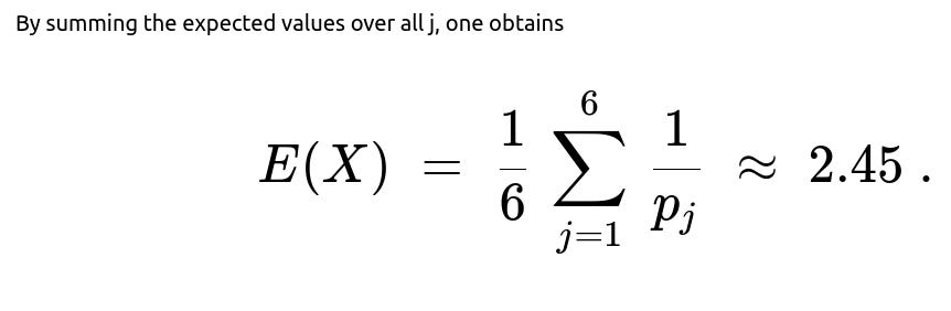
E(X) = (1/6) * Σ over j=1..6 of [1/p_j].

Substituting p_j = (6 - j + 1)/6, one can show that

E(X) = (1/6) * Σ over j=1..6 of [6 / (6 - j + 1)].

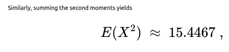
Numerical evaluation reveals E(X) ≈ 2.45. For the second moment E(X^2), one can use the known formula for the geometric distribution’s second moment:

E(X^2) = (2 - p) / p^2

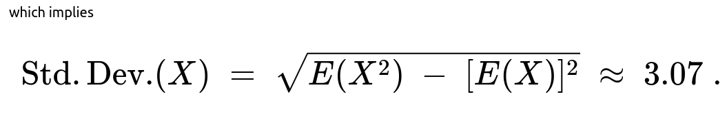
for a geometric distribution with parameter p. One then takes the average of these second moments across j. This gives E(X^2) ≈ 15.4467. Thus, the variance of X is 15.4467 - (2.45)^2 ≈ 9.4442, and the standard deviation is the square root of that, approximately 3.07.

Because this is a mixture of different geometric distributions with varying probabilities of success, it is reasonable that the overall standard deviation can be larger than the mean. When j is large, p_j is smaller, which increases the likelihood of longer waiting times, contributing significantly to the variance.

Follow-up question: Can we verify the result via a direct simulation in Python?

A straightforward way to confirm analytic results is to run many simulated trials and estimate the mean and standard deviation of X empirically. One can implement this using Python as follows:

import random
import statistics

def simulate_one_experiment():
    # Choose j uniformly from 1..6
    j = random.randint(1, 6)
    # Roll a fair die until outcome >= j
    roll_count = 0
    while True:
        roll_count += 1
        outcome = random.randint(1, 6)
        if outcome >= j:
            return roll_count

def run_simulation(num_experiments=10_000_00):
    results = []
    for _ in range(num_experiments):
        results.append(simulate_one_experiment())
    return statistics.mean(results), statistics.pstdev(results)

mean_est, std_est = run_simulation()
print("Estimated mean:", mean_est)
print("Estimated std dev:", std_est)

In this code, each experiment randomly selects j from the set {1, 2, 3, 4, 5, 6} with equal probability. It then rolls a fair die until a roll is at least j. The total number of rolls is recorded. Repeating a large number of times and taking the mean and standard deviation of the recorded values should yield approximate values near E(X) ≈ 2.45 and Std Dev(X) ≈ 3.07.

Follow-up question: Why is the mixture of geometric distributions relevant, and how does it affect the variance?

Because j is random, X is not just a single geometric distribution; rather it is selected from six distinct geometric distributions, each with a different success probability p_j. Some p_j values are relatively large (for smaller j), implying a smaller expected count of rolls, whereas others are small (for larger j), implying a larger expected count. This diversity amplifies the spread around the mean, hence producing a higher overall standard deviation than one might see in a single geometric distribution of similar mean.

Follow-up question: What if we used an alternative counting convention for the geometric distribution?

Sometimes the geometric distribution is defined to count the number of failures before the first success rather than the number of trials up to and including the first success. In that alternate definition, the parameter p remains the probability of success, but the formulas for the mean and variance change: the mean becomes (1 - p)/p and the variance (1 - p)/p^2. Hence it is important to clarify which version is being used. In this problem, it is explicit that we count the total number of rolls, including the successful one, so the formula for the mean is 1/p.

Follow-up question: Could we have approached this problem using unconditional probabilities directly, without conditioning on j?

It is possible but far more cumbersome, because one would have to account for all cases in which the die roll meets or exceeds each possible integer j. Directly leveraging conditional probabilities and known results about the geometric distribution is the more elegant approach. By conditioning on j first, the mathematics becomes straightforward, since each conditional scenario is a simple geometric waiting time.

Follow-up question: Are there any real-world applications of this type of mixed geometric scenario?

In real-world settings where a threshold is chosen at random and then a process continues until surpassing that threshold, such as random-time process completions or random acceptance levels, you can end up with a mixture distribution much like this one. It illustrates how variability in the threshold can significantly affect the distribution of the waiting time. Understanding the mixture approach helps accurately capture both the average waiting time and the distribution’s spread, which could be relevant in queueing theory, reliability engineering, or random acceptance sampling.

Below are additional follow-up questions

What if the die is not fair? How would that affect the probability mass function and the final results?

If the die is biased, the probability of rolling any particular face i (where i ranges from 1 to 6) is no longer 1/6. Suppose we define p_i = probability of rolling face i for i in {1, 2, 3, 4, 5, 6}, with the constraint that p_1 + p_2 + ... + p_6 = 1. When you pick j at random from {1..6}, you still do so with probability 1/6 for each j. However, once j is chosen, the probability of rolling a number greater than or equal to j is now p_j + p_{j+1} + ... + p_6. That new sum becomes the parameter for the geometric distribution that governs the number of rolls needed.

Thus, for a chosen j, the success probability becomes (p_j + p_{j+1} + ... + p_6). Let’s denote that sum by q_j. Then the distribution P(X = k | j) is q_j * (1 - q_j)^(k-1). The unconditional probability is

(1/6) * Σ over j=1..6 of [ q_j * (1 - q_j)^(k-1) ].

Likewise, the expectation E(X) is an average of 1/q_j over j, multiplied by 1/6. Specifically,

E(X) = (1/6) * Σ over j=1..6 of [1 / q_j].

You can see that if the die is heavily biased to favor large numbers, then for large j, q_j could become relatively large, which lowers the expected waiting time. Conversely, if the die is biased to favor smaller numbers, then for large j, q_j might be very small, leading to a large number of rolls.

A common subtlety arises if the candidate tries to use the unweighted formula 1/p_j from the fair scenario. That would be incorrect in the biased case because the success probability for each j changes. This is a pitfall when you see “geometric distribution” but fail to properly update the success parameter for each j under the bias. A thorough approach re-derives the success probabilities and sums them accordingly.

How would the result change if we want the die outcome to be strictly greater than the chosen integer j rather than greater or equal?

Currently, the success condition is “die roll ≥ j.” If we switch to “die roll > j,” then p_j for each j changes. Specifically, if j is chosen uniformly from 1..6, then:

• If j = 1, the die must be strictly greater than 1, so success is rolling {2, 3, 4, 5, 6}. Probability of success is 5/6.

• If j = 2, success is rolling {3, 4, 5, 6}, so probability is 4/6.

• Continuing in this manner, if j = 6, success is rolling only {7}, which is impossible, so the success probability is 0, meaning the number of rolls in that scenario becomes infinite in theory.

This last case is particularly interesting. Under “die roll > 6,” there is zero chance of success. Practically, that means that if j=6 happens and you are seeking strictly greater than 6, you never succeed. You might interpret that scenario as an infinite waiting time, or as “the event never occurs.” This would make the distribution ill-defined (you have a positive probability of j=6, leading to no possible success). If the problem is adjusted so that j is drawn from {1..5}, or the die is replaced with a bigger dice-like random variable, or you exclude j=6 from selection, then you can proceed with the same geometric mixture approach. But the presence of j=6 and “strictly greater than j” on a six-sided die is a corner case that can break the distribution (infinite expectation).

Hence, a subtle pitfall: if the problem statement modifies the inequality but still picks j=6 with nonzero probability, you must handle that scenario carefully, because you end up with a distribution that has infinite mean. This corner case shows why it is crucial to check each j in such mixture problems and see if success is even possible.

How can we find the cumulative distribution function (CDF) of X explicitly?

X is the total number of rolls needed to achieve a roll greater than or equal to j, with j chosen from 1..6. We know

P(X = k) = (1/6) * Σ over j=1..6 of [ p_j * (1 - p_j)^(k-1) ],

where p_j = (6 - j + 1)/6 in the fair-die scenario. To find P(X ≤ n), we sum k from 1 to n:

P(X ≤ n) = (1/6) * Σ over j=1..6 of Σ over k=1..n of [ p_j * (1 - p_j)^(k-1) ].

The inner sum Σ_{k=1..n} of [ p_j * (1 - p_j)^(k-1) ] is a finite geometric series. Specifically,

Σ_{k=1..n} [ p_j * (1 - p_j)^(k-1) ] = p_j * [ 1 - (1 - p_j)^n ] / p_j = 1 - (1 - p_j)^n.

So the CDF is

P(X ≤ n) = (1/6) * Σ_{j=1..6} [ 1 - (1 - p_j)^n ].

Hence,

P(X > n) = 1 - P(X ≤ n) = (1/6) * Σ_{j=1..6} [ (1 - p_j)^n ].

A hidden pitfall is mixing up the infinite series approach with the partial sum approach. Some might attempt to approximate the tail probability incorrectly. Using the direct geometric series approach helps avoid confusion and yields an explicit closed-form expression.

How would results change if you picked j from a non-uniform distribution over {1..6}?

So far we have assumed that j is chosen uniformly. Suppose instead that the probability of choosing j is w_j, where w_1 + w_2 + ... + w_6 = 1, but not necessarily each w_j = 1/6. Then the unconditional probability P(X = k) becomes a weighted sum:

P(X = k) = Σ_{j=1..6} [ w_j * p_j * (1 - p_j)^(k-1) ],

where p_j = (6 - j + 1)/6. The only difference is that each j is selected with probability w_j instead of 1/6. The expectation is

E(X) = Σ_{j=1..6} [ w_j * (1 / p_j) ].

You must make sure to incorporate the correct w_j for each j. A common error is to keep the 1/6 factor in the expression or to incorrectly apply the uniform assumption. Once w_j is changed, everything must be updated accordingly.

A subtle real-world edge case might be: you have some prior that j is more likely to be high or low. That shifts the distribution of waiting times because large j yields smaller success probability for each roll. This highlights how mixing distributions can shift the mean and variance considerably depending on your weighting function w_j.

How does introducing a maximum roll count or “cutoff” alter the analysis?

Imagine a scenario where you stop rolling if you reach some fixed cutoff M, regardless of whether you have succeeded by then. This means X is now bounded by M; if success occurs before M, you record that number of rolls, otherwise you record M (or consider it a “no success” outcome). The distribution is no longer purely geometric for each j because there is forced truncation.

Formally, for j chosen, let X_j be a geometric random variable with parameter p_j. Then the observed number of rolls Y_j is min(X_j, M). The unconditional distribution is the mixture of Y_j over j = 1..6. If M is large, Y_j mostly behaves like X_j except for small probability mass at M (the event that you never succeeded within M rolls). The expected number E(Y) = (1/6) * Σ_{j=1..6} E(min(X_j, M)) can be computed by summing P(X_j > k) for k from 0..M-1 or using known truncated geometric formulae.

A pitfall is assuming you can keep the same E(X_j) = 1/p_j when in fact there is a forced cap on the number of rolls. Another subtlety is that if M is small relative to the distribution’s tail, you get a large probability of hitting that maximum. This drastically changes both the distribution shape and the computed average. In real implementations (like bounded attempts in a system), ignoring the cutoff leads to incorrect predictions of system performance.

What if we only observe whether the number of rolls is even or odd, instead of the exact number?

In that case, we want P(X is even) and P(X is odd), or more precisely:

P(X is even) = Σ_{k = all even} P(X = k), P(X is odd) = Σ_{k = all odd} P(X = k).

Each P(X = k) is (1/6) * Σ_{j=1..6} [ p_j (1 - p_j)^(k-1) ]. We can sum separately for even k and odd k. Alternatively, there is a known approach for geometric distributions:

Let G(t) be the probability generating function for X. For a single geometric distribution with parameter p, G(t) = p t / (1 - (1 - p) t). You can then average this generating function over j, and evaluate at t = -1 to find P(X is even) - P(X is odd), or do partial expansions. However, you must be mindful that in the mixture setting, you have an average of generating functions. The partial sums approach might be simpler:

P(X is even) = Σ_{k=1..∞} [P(X=2k)], P(X is odd) = Σ_{k=1..∞} [P(X=2k-1)].

Though this is not typically requested, it illustrates how you can combine mixture distributions and known summation tricks. A pitfall is forgetting that you must sum over j inside each term. Another is incorrectly applying the geometric distribution’s even-odd expansions without weighting them by 1/6 for each j.

Could there be any correlation issue if we run multiple experiments where we choose j each time?

Each experiment is presumably independent: we choose j once from the uniform distribution for that experiment, then keep rolling until we get a roll ≥ j. That process resets each time. Therefore, if we do multiple trials, the results across different experiments are uncorrelated, since the choice of j in each trial is independent of previous trials and the dice rolls in each trial are also independent.

A subtlety might arise if a real-world scenario does not properly randomize j for each new experiment or if the same die faces might be “sticky” across experiments (for instance, a physical die becoming worn out, changing the probabilities). In theoretical settings we ignore that. Another subtle point is whether partial knowledge of previous outcomes might change how j is chosen in subsequent experiments, creating correlation between X-values across trials. That would invalidate the assumption of independence. However, under the standard statement of the problem, there is no correlation: each trial stands alone, and the mixture distribution analysis remains valid.