
ML Interview Q Series: Geometric Probability: Point Distance to Nearest Rectangle Side

Browse all the Probability Interview Questions here.
You choose at random a point inside a rectangle whose sides have lengths 2 and 3. For 0 < a < 1, what is the probability that the distance of the point to the closest side is no more than a?
Short Compact solution
Consider the rectangle 0 <= x <= 3 and 0 <= y <= 2. Define A to be the set of points inside this rectangle whose distance to the closest side is larger than a. Geometrically, these points form a smaller rectangle of dimensions (3 - 2a) by (2 - 2a). Hence the area of A is (3 - 2a)(2 - 2a). Consequently, the region of interest (points whose distance to the closest side is no more than a) is the complement of A in the original 3-by-2 rectangle. Since the total area is 6, the probability is:
Comprehensive Explanation
Understanding the geometric setup
The rectangle is 3 units wide (x-direction) and 2 units tall (y-direction). A point chosen uniformly inside this rectangle has coordinates (x, y) with x in [0, 3] and y in [0, 2]. We want the probability that this point’s distance to the closest side is at most a, for 0 < a < 1.
In two dimensions, the distance to the closest side of a rectangular region is the minimum of:
Distance to the left edge (which is x)
Distance to the right edge (which is 3 - x)
Distance to the bottom edge (which is y)
Distance to the top edge (which is 2 - y)
A point has a distance to the closest side greater than a if it is at least a units away from all four edges. Visualizing this, you obtain a smaller “inner” rectangle offset from each edge by a margin of length a. The smaller rectangle therefore has width 3 - 2a and height 2 - 2a.
Key steps
Calculate the area of the original rectangle: 6.
The set of points whose distance to any side is greater than a is a smaller rectangle with area (3 - 2a)(2 - 2a).
The probability that the distance is greater than a is that smaller area divided by 6.
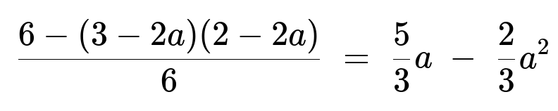
Therefore, the probability that the distance is no more than a is 1 minus the above ratio, giving:
(6 - (3 - 2a)(2 - 2a)) / 6
Expand (3 - 2a)(2 - 2a) = 6 - 6a - 4a + 4a^2 = 6 - 10a + 4a^2, and subtract from 6 to get 6 - (6 - 10a + 4a^2) = 10a - 4a^2.
Divide by 6: (10a - 4a^2) / 6 = (5/3)a - (2/3)a^2.
This matches the final expression. It also aligns with intuitive boundary checks:
If a is very small (close to 0), the probability is near 0.
If a is close to 1, nearly the entire rectangle is within distance 1 of some side, so the probability approaches 1.
Implementation using a simulation approach
Below is an example in Python where we can approximate the probability numerically by random sampling. When we run this code repeatedly for a given a, it should converge near (5/3)a - (2/3)a^2.
import random

def estimate_probability(a, trials=10_000_000):
    count = 0
    for _ in range(trials):
        x = 3 * random.random()
        y = 2 * random.random()
        dist_to_closest_side = min(x, 3 - x, y, 2 - y)
        if dist_to_closest_side <= a:
            count += 1
    return count / trials

# Example usage:
a_value = 0.5
approx_prob = estimate_probability(a_value)
print(f"Approximate Probability for a={a_value}: {approx_prob}")
The result of approx_prob should be close to (5/3)*0.5 - (2/3)*0.5^2 = 5/6 - 2/12 = 5/6 - 1/6 = 4/6 = 2/3.
Follow-Up Question 1
Why must a be strictly less than 1 for this formula to hold, and what happens if a = 1?
It is crucial that a be strictly less than 1 to ensure that the “inner” rectangle has nonnegative dimensions 3 - 2a and 2 - 2a. If a were bigger than 1, the quantity 2 - 2a would become negative (because 2 - 2(1.1) = 2 - 2.2 = -0.2, for example), which would not make sense for the rectangle’s dimensions.
However, when a = 1, it precisely covers every point in the rectangle, because the farthest distance a point can have from one of the edges in a 2-by-3 rectangle is at most 1 along the shorter side (the maximum distance from top or bottom edges is 1). Hence, the probability becomes 1 if a is exactly 1, which is consistent with plugging a = 1 into the expression (5/3) a - (2/3) a^2 = 1.
Follow-Up Question 2
What if we have a general rectangle of length L and width W instead of 3 and 2?
The generalization is straightforward. The total area is L * W. The points whose distance to the closest side is larger than a form a rectangle with dimensions (L - 2a) and (W - 2a). The probability that a random point lies within distance a of a side is:
1 - ( (L - 2a)(W - 2a) ) / (L * W),
as long as L > 2a and W > 2a. If L <= 2a or W <= 2a, the probability that the point is no more than a units from a side becomes 1, because the entire rectangle is covered.
Follow-Up Question 3
How would you derive or interpret the distribution of “distance from the closest side” for a random point?
To find this distribution explicitly, one would note that the distance to the closest side is a random variable d ranging from 0 up to min(W/2, L/2). One can break this down by integrating over the “shells” in the rectangle that are at a constant distance x from any side. Each such shell has a particular perimeter-like shape, and by computing the differential area, we can determine the probability density function. Conceptually, as x grows from 0 to some maximum, the “shell” is effectively the boundary of the smaller rectangle offset by x from all sides.
This involves more advanced geometric integration, but the end result is consistent with the probabilities we computed: we can always integrate the probability that d <= a, resulting in the area-based expression we used.
Follow-Up Question 4
What practical issues might arise when simulating this probability for very small or very large a?
If a is extremely small, the probability is also small. In a simulation, you might need a large number of random draws to reliably estimate a small probability because the number of “successes” (points within distance a of a side) can be quite small, increasing variance.
On the other hand, if a is close to 1, you might get nearly all samples satisfying the condition. This again requires a sufficiently large sample size to distinguish the probability from 1. If you do not choose enough samples, your simulation might be biased due to how random fluctuations manifest near the boundaries of the rectangle. Proper random seeding and large trial counts help mitigate such issues.
Below are additional follow-up questions
Follow-up Question 1
What if the rectangle is tilted at some arbitrary angle relative to the coordinate axes? How would we adapt the approach or formula to this scenario?
Even if the rectangle is rotated, the fundamental idea still applies: the distance to the closest side of the rectangle is the minimum distance to one of its four line segments. If we know the orientation (e.g., the rectangle is defined by its vertices), we could:
Transform coordinates to an axis-aligned system. One way is to apply a 2D rotation that aligns the rectangle edges with the axes. After such a rotation, the problem becomes equivalent to the axis-aligned case.
In that transformed coordinate space, the rectangle looks just like the original 3-by-2 or L-by-W rectangle, and we can use the same geometric offset approach: the “inner rectangle” that is a distance a from each side.
Transform back if needed. For probability calculations, the rotation does not change the uniform distribution area argument; area is preserved under rigid transformations.
Potential pitfalls:
If the rectangle is not strictly convex (e.g., if we had a more complicated polygon or shape), simply offsetting edges might create additional internal boundaries, so care must be taken.
Handling very small angles of rotation can introduce floating-point inaccuracies if you attempt to numerically compute distances from each side in an untransformed coordinate system.
Follow-up Question 2
How would this change if the rectangle has “rounded corners” or if we have a shape that is nearly rectangular but not perfectly?
If you have a shape that is “almost” a rectangle but with slight curves or irregular edges (for instance, a stadium shape with rounded corners), you cannot rely on the simple inner rectangle offset by a. Instead:
You would define the region of points that lie within distance a of any boundary. Mathematically, this is akin to expanding (or shrinking) the polygon by a constant width. For rectangles with rounded corners, these expansions or contractions involve arcs at the corners rather than sharp 90-degree corners.
The area-based probability would need to integrate over curved boundary regions. In general, it is more complex to compute analytically.
Approximate numerical approaches—such as Monte Carlo sampling or computational geometry libraries—often become the more practical solution.
Potential pitfalls:
Failing to account for curvature at corners could produce an overestimate or underestimate of the region.
In real-world engineering problems (e.g., robotic motion planning near walls), ignoring these small corner effects can lead to collisions because the shape’s boundary is not strictly rectangular.
Follow-up Question 3
Could this probability be generalized to higher dimensions, say a 3D cuboid, to compute the probability that a randomly chosen point is within distance a of any face?
Yes. In three dimensions, you would have a cuboid of dimensions X, Y, Z. A point is within distance a of the nearest face if at least one coordinate is within a of 0 or the maximum dimension in that coordinate. Specifically:
The region of points where the distance to every face is more than a is a smaller cuboid of dimension (X - 2a) x (Y - 2a) x (Z - 2a), provided X > 2a, Y > 2a, Z > 2a.
So, the volume of this region is (X - 2a)(Y - 2a)(Z - 2a).
The probability that a random point in the original cuboid is more than a units away from every face is that smaller volume divided by the total volume XYZ.
Consequently, the probability of being within distance a of at least one face is 1 - [(X - 2a)(Y - 2a)(Z - 2a)] / (X Y Z).
Potential pitfalls:
If a is large enough such that X - 2a < 0 (or Y - 2a < 0, etc.), then the smaller cuboid collapses, and the probability becomes 1.
Computational geometry in 3D can get complicated when dealing with edges and corners if the shape is not strictly rectangular (e.g., with complicated polyhedra).
Follow-up Question 4
What happens if we allow a to be a random variable instead of a fixed number?
In some scenarios, “a” might be drawn from a probability distribution (e.g., a is random). Then the probability we want is the expectation over all possible a values:
P(distance to side ≤ a) = integral of [ P(distance to side ≤ x) ] f(x) dx,
where f(x) is the probability density function for a. Concretely:
If we have a known distribution for a, we can integrate or sum the result (5/3 x - 2/3 x^2) with respect to that distribution in the domain where the formula is valid (0 < x < 1 for the 3-by-2 rectangle).
Alternatively, a sampling approach can be used: For each random draw of a, you compute the geometric probability, and average the result.
Potential pitfalls:
If a’s distribution allows values >= 1 frequently, the probability that the distance is within a is automatically 1 for those draws. This can skew the results if not accounted for.
Numerical approximation might require large sample sizes, especially if the distribution of a is broad.
Follow-up Question 5
How does one approach verifying the correctness of the analytical probability expression outside of a purely uniform random model, for instance if points are distributed non-uniformly?
Our derivation assumes a uniform distribution over the rectangle. If the distribution is not uniform, e.g., weighted more heavily in one corner, then:
The probability is no longer simply “(area of region) / (total area).” Instead, you must integrate the probability density over the subset that is within distance a of a side.
You can define a density function p(x, y) over the rectangle. Then, the probability that the point lies in the region within distance a of a side is the integral ∫∫ p(x, y) dx dy, taken over that region.
To check correctness, you could sample from the given non-uniform distribution (e.g., using acceptance-rejection methods) and empirically measure how many points lie within distance a of a side.
Potential pitfalls:
Misidentifying a distribution as uniform when it is not, leading to an incorrect simple area ratio.
Properly discretizing or integrating the density in complicated shapes near corners or edges, which might require higher grid resolution in a numerical method.
Follow-up Question 6
Can we estimate the probability to within a certain error margin efficiently, and what computational or numerical methods could we use?
Yes, both analytical and numerical approaches can control error margins. For instance:
Monte Carlo simulation: By increasing the number of draws N, you reduce the standard error (proportional to 1/√N). Carefully manage the random seeds and incorporate variance-reduction techniques (e.g., antithetic sampling or stratified sampling) if you need faster convergence.
Quasi-Monte Carlo methods: Using low-discrepancy sequences like Sobol or Halton can improve convergence rates, especially in higher dimensions or more complex geometry.
Deterministic numerical approximation: For more complex shapes, you might discretize the domain into small cells and approximate the distance to the nearest boundary. Summing up the cells that satisfy the distance constraint, multiplied by the cell area, provides an approximate measure.
Potential pitfalls:
For small a, you need finer sampling near the edges, or else your estimates may be biased.
For large a that approaches 1, near-complete coverage of the rectangle can lead to numerical saturation (e.g., you always see successes in simulation). You need enough trials to accurately capture the slight difference from the full area.
In high-dimensional analogs, naive Monte Carlo might converge too slowly without specialized variance-reduction methods.